Isotope Fingerprinting

Last updated

Mar 14, 2023
Save as PDF
- Glass Density Evidence
- Geology

$\newcommand{\vecs}[1]{\overset { \scriptstyle \rightharpoonup} {\mathbf{#1}} }$

$\newcommand{\vecd}[1]{\overset{-\!-\!\rightharpoonup}{\vphantom{a}\smash {#1}}}$

$\newcommand{\id}{\mathrm{id}}$ $\newcommand{\Span}{\mathrm{span}}$

( \newcommand{\kernel}{\mathrm{null}\,}\) $\newcommand{\range}{\mathrm{range}\,}$

$\newcommand{\RealPart}{\mathrm{Re}}$ $\newcommand{\ImaginaryPart}{\mathrm{Im}}$

$\newcommand{\Argument}{\mathrm{Arg}}$ $\newcommand{\norm}[1]{\| #1 \|}$

$\newcommand{\inner}[2]{\langle #1, #2 \rangle}$

$\newcommand{\Span}{\mathrm{span}}$

$\newcommand{\id}{\mathrm{id}}$

$\newcommand{\Span}{\mathrm{span}}$

$\newcommand{\kernel}{\mathrm{null}\,}$

$\newcommand{\range}{\mathrm{range}\,}$

$\newcommand{\RealPart}{\mathrm{Re}}$

$\newcommand{\ImaginaryPart}{\mathrm{Im}}$

$\newcommand{\Argument}{\mathrm{Arg}}$

$\newcommand{\norm}[1]{\| #1 \|}$

$\newcommand{\inner}[2]{\langle #1, #2 \rangle}$

$\newcommand{\Span}{\mathrm{span}}$ $\newcommand{\AA}{\unicode[.8,0]{x212B}}$

$\newcommand{\vectorA}[1]{\vec{#1}} % arrow$

$\newcommand{\vectorAt}[1]{\vec{\text{#1}}} % arrow$

$\newcommand{\vectorB}[1]{\overset { \scriptstyle \rightharpoonup} {\mathbf{#1}} }$

$\newcommand{\vectorC}[1]{\textbf{#1}}$

$\newcommand{\vectorD}[1]{\overrightarrow{#1}}$

$\newcommand{\vectorDt}[1]{\overrightarrow{\text{#1}}}$

$\newcommand{\vectE}[1]{\overset{-\!-\!\rightharpoonup}{\vphantom{a}\smash{\mathbf {#1}}}}$

$\newcommand{\vecs}[1]{\overset { \scriptstyle \rightharpoonup} {\mathbf{#1}} }$

$\newcommand{\vecd}[1]{\overset{-\!-\!\rightharpoonup}{\vphantom{a}\smash {#1}}}$

$\newcommand{\avec}{\mathbf a}$

$\newcommand{\bvec}{\mathbf b}$

$\newcommand{\cvec}{\mathbf c}$

$\newcommand{\dvec}{\mathbf d}$

$\newcommand{\dtil}{\widetilde{\mathbf d}}$

$\newcommand{\evec}{\mathbf e}$

$\newcommand{\fvec}{\mathbf f}$

$\newcommand{\nvec}{\mathbf n}$

$\newcommand{\pvec}{\mathbf p}$

$\newcommand{\qvec}{\mathbf q}$

$\newcommand{\svec}{\mathbf s}$

$\newcommand{\tvec}{\mathbf t}$

$\newcommand{\uvec}{\mathbf u}$

$\newcommand{\vvec}{\mathbf v}$

$\newcommand{\wvec}{\mathbf w}$

$\newcommand{\xvec}{\mathbf x}$

$\newcommand{\yvec}{\mathbf y}$

$\newcommand{\zvec}{\mathbf z}$

$\newcommand{\rvec}{\mathbf r}$

$\newcommand{\mvec}{\mathbf m}$

$\newcommand{\zerovec}{\mathbf 0}$

$\newcommand{\onevec}{\mathbf 1}$

$\newcommand{\real}{\mathbb R}$

$\newcommand{\twovec}[2]{\left[\begin{array}{r}#1 \\ #2 \end{array}\right]}$

$\newcommand{\ctwovec}[2]{\left[\begin{array}{c}#1 \\ #2 \end{array}\right]}$

$\newcommand{\threevec}[3]{\left[\begin{array}{r}#1 \\ #2 \\ #3 \end{array}\right]}$

$\newcommand{\cthreevec}[3]{\left[\begin{array}{c}#1 \\ #2 \\ #3 \end{array}\right]}$

$\newcommand{\fourvec}[4]{\left[\begin{array}{r}#1 \\ #2 \\ #3 \\ #4 \end{array}\right]}$

$\newcommand{\cfourvec}[4]{\left[\begin{array}{c}#1 \\ #2 \\ #3 \\ #4 \end{array}\right]}$

$\newcommand{\fivevec}[5]{\left[\begin{array}{r}#1 \\ #2 \\ #3 \\ #4 \\ #5 \\ \end{array}\right]}$

$\newcommand{\cfivevec}[5]{\left[\begin{array}{c}#1 \\ #2 \\ #3 \\ #4 \\ #5 \\ \end{array}\right]}$

$\newcommand{\mattwo}[4]{\left[\begin{array}{rr}#1 \amp #2 \\ #3 \amp #4 \\ \end{array}\right]}$

$\newcommand{\laspan}[1]{\text{Span}\{#1\}}$

$\newcommand{\bcal}{\cal B}$

$\newcommand{\ccal}{\cal C}$

$\newcommand{\scal}{\cal S}$

$\newcommand{\wcal}{\cal W}$

$\newcommand{\ecal}{\cal E}$

$\newcommand{\coords}[2]{\left\{#1\right\}_{#2}}$

$\newcommand{\gray}[1]{\color{gray}{#1}}$

$\newcommand{\lgray}[1]{\color{lightgray}{#1}}$

$\newcommand{\rank}{\operatorname{rank}}$

$\newcommand{\row}{\text{Row}}$

$\newcommand{\col}{\text{Col}}$

$\renewcommand{\row}{\text{Row}}$

$\newcommand{\nul}{\text{Nul}}$

$\newcommand{\var}{\text{Var}}$

$\newcommand{\corr}{\text{corr}}$

$\newcommand{\len}[1]{\left|#1\right|}$

$\newcommand{\bbar}{\overline{\bvec}}$

$\newcommand{\bhat}{\widehat{\bvec}}$

$\newcommand{\bperp}{\bvec^\perp}$

$\newcommand{\xhat}{\widehat{\xvec}}$

$\newcommand{\vhat}{\widehat{\vvec}}$

$\newcommand{\uhat}{\widehat{\uvec}}$

$\newcommand{\what}{\widehat{\wvec}}$

$\newcommand{\Sighat}{\widehat{\Sigma}}$

$\newcommand{\lt}{<}$

$\newcommand{\gt}{>}$

$\newcommand{\amp}{&}$

$\definecolor{fillinmathshade}{gray}{0.9}$

"A single hair can determine a person's location during the past weeks or even years" (Thure E. Cerling). Hair analysis has been used to solve several murders through geographical tracking.

Diagram of a hair follicle showing hair, skin surface, sebum, follicle, and the sebaceous gland. — Figure $\PageIndex{1}$ : *A hair follicle*

What sort of forensics tests can determine geographic location from a hair?

The technique is called stable isotope analysis or Isotope Fingerprinting. The element hydrogen has two stable isotopes ( $\ce{^1_1H}$ and $\ce{^2_1H}$ ) and the element oxygen has three ( 168O, 178O, 188O) in addition to their several radioactive isotopes. The stable isotopes are found in various ratios, or "isotopic signatures" which vary depending on the source. Biological processes, as well as evaporation and other physical processes, often yield products with distinctive isotopic ratios. Isotopic fingerprinting of materials is used increasingly in forensics, to determine the origin of otherwise similar materials and tracking materials to their common source. There is a Forensic Isotope Ratio Mass Spectrometry (FIRMS) Network devoted to the field, and annual meetings of investigators.

Isotope "delta" Values

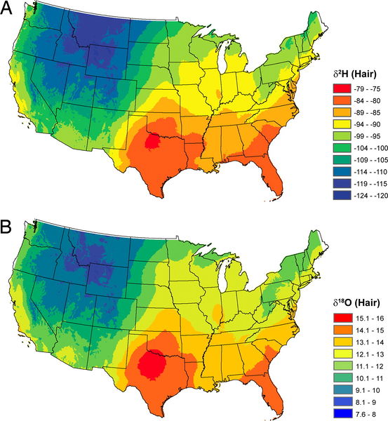
Thure Cerling discovered that a single hair could provide evidence to where a person lived (and even when that person lived there). The analysis is based on "δ²H" and "δ¹⁸O" values. The table below shows typical geographical ranges of these delta values for drinking water (δ²H_dw and δ¹⁸O_dw), as well as for hair, oxygen in the air (O₂), and food. The delta value for food does not vary much from place to place, because of our "continental supermarket" where essentially all foods come from the same sources. Delta values represent very small differences in isotopic ratios, so they're measured in parts per thousand (or "per mil", ‰), and the more negative the value, the more of the lighter isotope is present, so positive values represent material with more of the heavy isotope. You can see that isotopic abundances vary widely from place to place or sample to sample.

Table $\PageIndex{1}$ Isotope Ratios
Isotope Ratio	Value	Isotope Ratio	Value
δ²H_dw heaviest, Montana	+4‰	δ¹⁸O_hair(heaviest)	+15.9‰
δ²H_dw lightest, Oklahoma	-140‰	δ¹⁸O_hair (lightest)	+7.4‰
δ¹⁸O_dw heaviest, Montana	+1.3‰	δ²H_food	-115‰
δ¹⁸O_dw lightest, Oklahoma	-18‰	δ¹⁸O_food	+25‰
δ²H_hair heaviest	-77‰	δ¹⁸O_O₂	+23.5‰
δ²H_hair lightest	-125‰

Figure

The details of the delta value calculations are not important, but in case you're interested, the formula is

But is there a "normal" isotopic abundance ratio for an element? If the abundance of oxygen isotopes can vary by ~20‰ (2%), how can we have a single "atomic weight" for the element?

The "Normal" Isotopic Ratio: Atomic Weights

All atoms of a given element do not necessarily have identical masses. But all elements combine in definite mass ratios, so they behave as if they had just one kind of atom. In order to solve this dilemma, we define the atomic weight as the weighted average mass of all naturally occurring (occasionally radioactive) isotopes of the element.

A weighted average is defined as

$\text{Atomic Weight} = \left(\dfrac{\%\text{ abundance isotope 1}}{100}\right)\times \left(\text{mass of isotope 1}\right) + \left(\dfrac{\%\text{ abundance isotope 2}}{100}\right)\times \left(\text{mass of isotope 2}\right) + ...$

Similar terms would be added for all the isotopes. Since the abundances change from place to place, IUPAC has established "normal" abundances which are most likely to be encountered in the laboratory. This important document that reports these values can be found at the IUPAC site. The abundances are also usually listed on the Table of the Nuclides which lists all isotopes for all elements. Surprisingly, a good number of elements have isotopic abundances that vary quite widely, so that atomic weights based on them have only 3 or 4 digit precision.

The atomic weight calculation is analogous to the method used to calculate grade point averages in most colleges:

$\text{GPA} = \left(\dfrac{\text{Credit Hours Course 1}}{\text{total credit hours}}\right)\times \left(\text{Grade in Course 1}\right) + \left(\dfrac{\text{Credit Hours Course 2}}{\text{total credit hours}}\right)\times \left(\text{Grade in Course 2}\right) + ...$

Example $\PageIndex{1}$ : The Atomic Weight of Oxygen

The IUPAC Report gives the following data for oxygen:

99.757% ${}_{\text{8}}^{\text{16}}\text{O}$ whose isotopic weight is 15.9949146.
0.038% ${}_{\text{8}}^{\text{17}}\text{O}$ whose isotopic weight is 16.9991315 .
0.205% ${}_{\text{8}}^{\text{18}}\text{O}$ whose isotopic weight is 17.9991604.

Calculate the atomic weight of an average naturally occurring sample of carbon.

Solution

$\dfrac{\text{99.757}}{\text{100.00}} \times \text{15.9949} + \dfrac{\text{0.038}}{\text{100.00}} \times \text{16.99913} + \dfrac{\text{0.205}}{\text{100.00}} \times \text{17.99916} = \text{15.9994} \nonumber$

Hair Isotope Analysis

While we use the "normal" 99.757% abundance for ${}_{\text{8}}^{\text{16}}\text{O}$ to calculate the standard atomic weight, the abundance varies from 99.7384% - 99.7756% (other oxygen isotope abundances vary similarly). This allows the "isotopic fingerprinting" discussed above.

Hair is mostly a protein called keratin, so the mechanism by which ${}_{\text{8}}^{\text{18}}\text{O}$ or ${}_{\text{1}}^{\text{2}}\text{H}$ might be incorporated into the protein is of interest. Apparently, when plant or animal protein is digested in the gut, the drinking water that is also present can be incorporated into the individual amino acids that result when the protein is hydrolyzed. The amino acids are then incorporated into keratin. ${}_{\text{1}}^{\text{2}}\text{H}$ is probably incorporated in the hair follicle, because acidic protons on the keratin exchange with water protons.

Since we are all exposed to the same atmospheric oxygen and food (which have constant isotopic ratios), the isotopic ratios of drinking water determine the ratios in hair (the ratio in hair is not the same, but is proportional to, the drinking water ratio).

To establish this relationship, samples of tap water were collected from more than 600 cities across the United States. Hair samples were collected from the barbershops in 65 cities in 20 states.

Example $\PageIndex{1}$ : Atomic Weight of Hydrogen

Naturally occurring hydrogen is found to consist of two isotopes:

99.9885% ${}_{\text{1}}^{\text{1}}\text{H}$ whose isotopic weight is 1.007825 . 0.01 15% ${}_{\text{1}}^{\text{2}}\text{H}$ whose isotopic weight is 2.01410178 .

Calculate the atomic weight of an average naturally occurring sample of hydrogen.

Atomic Weight =

$\dfrac{\text{99.9885}}{\text{100.00}} \times \text{1.00782503207 amu} + \dfrac{\text{0.0115}}{\text{100.00}} \times \text{2.0141017778 amu} + \dfrac{0}{\text{100.00}} \times \text{3.016049277} = \text{1.00794 amu}$

Defining the Mole

The SI definition of the mole also depends on the isotope ${}_{\text{6}}^{\text{12}}\text{C}$ and can now be stated. One mole is defined as the amount of substance of a system which contains as many elementary entities as there are atoms in exactly 0.012 kg of 126C. The elementary entities may be atoms, molecules, ions, electrons, or other microscopic particles. This official definition of the mole makes possible a more accurate determination of the Avogadro constant than was reported earlier. The currently accepted value is N_A = 6.02214179 × 10²³ mol^–1. This is accurate to 0.00000001 percent and contains five more significant figures than 6.022 × 10²³ mol^–1, the number used to define the mole previously. It is very seldom, however, that more than four significant digits are needed in the Avogadro constant. The value 6.022× 10²³ mol^–1 will certainly suffice for most calculations needed.

From ChemPRIME: 4.13: Average Atomic Weights

References

http://en.Wikipedia.org/wiki/Thure_E._Cerling
http://en.Wikipedia.org/wiki/Isotope_analysis#Forensics
http://www.pnas.org/content/105/8/2788.full
http://www.rsc.org/chemistryworld/News/2008/February/26020801.asp
Data from http://www.pnas.org/content/105/8/2788.full)
James R. Ehleringer*†‡, Gabriel J. Bowen†§, Lesley A. Chesson*†, Adam G. West†¶, David W. Podlesak*, and Thure E. Cerling*†‡ Hydrogen and oxygen isotope ratios in human hair are related to geography 2788–2793 _ PNAS _ February 26, 2008 _ vol. 105 _ no. 8;

Contributors and Attributions

Ed Vitz (Kutztown University), John W. Moore (UW-Madison), Justin Shorb (Hope College), Xavier Prat-Resina (University of Minnesota Rochester), Tim Wendorff, and Adam Hahn.

Search

Text Color

Text Size

Margin Size

Font Type