5.6: The Wavefunction and Schrödinger's Equation

Estimated Time to Read: 6 min

Quantum Mechanics

Electrons and other subatomic particles behave as both particles and waves. An individual particle like an electron has mass, but it is spread out, not located in one position, and it has a wavelength. The wavelike nature of electrons and other subatomic particles, as well as the paradox described by Heisenberg’s uncertainty principle, made it impossible to use the equations of classical physics to describe the motion of electrons in atoms. Scientists needed a new approach that took the wave behavior of the electron into account.

In 1926, an Austrian physicist, Erwin Schrödinger (1887–1961; Nobel Prize in Physics, 1933), developed wave mechanics, a mathematical technique that describes the relationship between the motion of a particle that exhibits wavelike properties and its allowed energies. Schrödinger's wave equation allowed scientists to make predictions about the electronic structure of atoms. Where are the electrons found? What is their energy?

Although quantum mechanics uses sophisticated mathematics, you do not need to understand the mathematical details to follow our discussion of its general conclusions. We focus on the properties of the wavefunctions that are the solutions of Schrödinger’s equations.

Erwin Schrödinger (1887–1961)

Schrödinger’s unconventional approach to atomic theory was typical of his unconventional approach to life. He was notorious for his intense dislike of memorizing data and learning from books. When Hitler came to power in Germany, Schrödinger escaped to Italy. He then worked at Princeton University in the United States but eventually moved to the Institute for Advanced Studies in Dublin, Ireland, where he remained until his retirement in 1955.

Wavefunctions

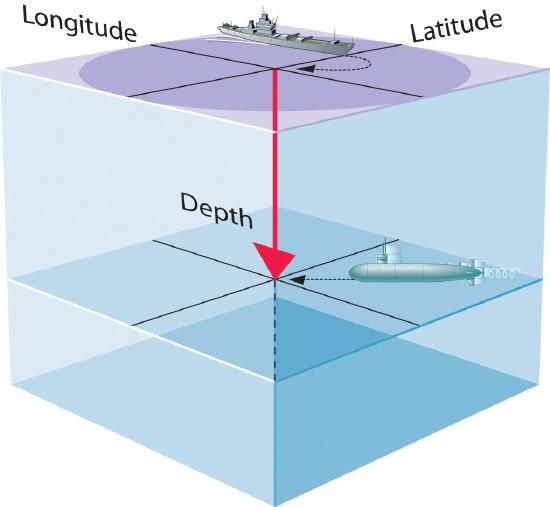
A wavefunction (Ψ) is a mathematical function that relates the location of an electron and the energy of the electron. A wavefunction uses three variables to describe the position of an electron in space (as with the Cartesian coordinates x, y, and z). A fourth variable specifies the time at which the electron is at the specified location.

By analogy, if you were the captain of a ship trying to intercept an enemy submarine, you would need to know its latitude, longitude, and depth, as well as the time at which it was going to be at this position (Figure \(\PageIndex{1}\)). For electrons, we can ignore the time dependence because we will be using standing waves, which by definition do not change with time, to describe the position of an electron.

Figure \(\PageIndex{1}\): The Four Variables (Latitude, Longitude, Depth, and Time) required to precisely locate an object

The magnitude of the wavefunction at a particular point in space is proportional to the amplitude of the wavefunction at that point. Many wavefunctions are complex functions, which means that they contain \(\sqrt{-1}\), represented as \(i\). Hence the amplitude of the wave has no real physical significance.

In contrast, the sign of the wavefunction (either positive or negative) corresponds to the phase of the wave, which will be important in our discussion of chemical bonding. The sign of the wavefunction should not be confused with a positive or negative electrical charge.

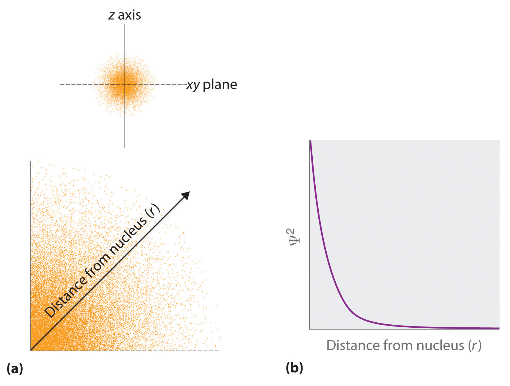
The square of the wavefunction at a given point in space is proportional to the probability of finding an electron at that point in space. (The square of the wavefunction (\(\Psi^2\)) is always a real quantity [recall that that \(\sqrt{-1}^2=-1\)]) The probability of finding an electron at any point in space depends on several factors, including the distance from the nucleus and, in many cases, the atomic equivalent of latitude and longitude. One way of graphically representing the probability distribution is demonstrated in Figure \(\PageIndex{2}\) for a hydrogen atom. The probability of finding an electron is indicated by the density of colored dots.

Schrödinger’s approach treats electrons as three-dimensional standing waves. It is a requirement of standing waves that they be in phase with one another to avoid cancellation; this results in a limited number of solutions (wavefunctions), each of which is associated with a particular energy. As in Bohr’s model, the energy of an electron in an atom is quantized; it can have only certain allowed values, which are specified by the quantum numbers. Quantum numbers define solutions to the Schrödinger equation. The major difference between Bohr’s model and Schrödinger’s approach is that Bohr had to impose the idea of quantization arbitrarily, whereas in Schrödinger’s approach, quantization is a natural consequence of describing an electron as a standing wave.

Figure \(\PageIndex{2}\): Probability of Finding the Electron in the Ground State of the Hydrogen Atom at Different Points in Space. (a) The density of the dots shows electron probability. (b) In this plot of Ψ² versus r for the ground state of the hydrogen atom, the electron probability density is greatest at r = 0 (the nucleus) and falls off with increasing r. Because the line never actually reaches the horizontal axis, the probability of finding the electron at very large values of r is very small but not zero.

The wavefunction is a mathematical expression that describes the electron. It can be plotted as a three-dimensionional graph. The three-dimensional plot of the wavefunction is sometimes called an orbital. Often, chemists find it useful to look at pictures of orbitals in order to gain some sense of where electrons may be and how they may behave. In another sense, orbitals are probability maps that reveal the probability of an electron being located at a particular position in space.

Suppose you could take a series of photos of an electron and superimpose all of those pictures, like time-lapse photography. The result might look something like the drawing in Figure \(\PageIndex{2}\), in which every dot represents where the electron showed up in one of the photos. It's impossible to predict exactly where the electron would show up in the next photo, but it would be a pretty good guess that it would show up somewhere in the same rough circle as it did all of the other times.

Figure \(\PageIndex{3}\): Probability map, or orbital, of a wavefunction. Each dots represents the probability of an electron being located at that point in space at a moment in time. (https://employees.csbsju.edu/cschall...tomnumbers.htm; Chris Schaller)

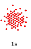
In three-dimensional space, the probability map, or orbital (named in reference to the Bohr Model) shown in Figure \(\PageIndex{3}\) would be a sphere instead of a circle. The probability map shown can be interpreted as a thin slice through the middle of the probability sphere. The orbital shown is specifically an s orbital. In the very center of the sphere, is the nucleus of the atom. The electron is found within a certain distance of the nucleus, but it can be found in any direction. Other electrons will have different distributions about the nucleus of the atom, resulting in other orbital shapes in three-dimensional space. Quantum numbers will be used to describe the various orbitals, the probability of finding an electron at a point in space and roughly how much energy the electron has.