5.4: Line Spectra and the Bohr Model

Learning Objectives

• Describe the relationship between atomic spectra and the electronic structure of atoms
• Describe the Bohr model of the hydrogen atom
• Use the Rydberg equation to calculate energies of light emitted or absorbed by hydrogen atoms

The concept of the photon emerged from experimentation with thermal radiation, electromagnetic radiation emitted as the result of a source’s temperature, which produces a continuous spectrum of energies.The photoelectric effect provided indisputable evidence for the existence of the photon and thus the particle-like behavior of electromagnetic radiation. However, more direct evidence was needed to verify the quantized nature of energy in all matter. In this section, we describe how observation of the interaction of atoms with visible light provided this evidence.

Line Spectra

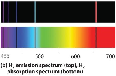
Although objects at high temperature emit a continuous spectrum of electromagnetic radiation, a different kind of spectrum is observed when pure samples of individual elements are heated. For example, when a high-voltage electrical discharge is passed through a sample of hydrogen gas at low pressure, the resulting individual isolated hydrogen atoms caused by the dissociation of H₂ emit a red light. Unlike blackbody radiation, the color of the light emitted by the hydrogen atoms does not depend greatly on the temperature of the gas in the tube. When the emitted light is passed through a prism, only a few narrow lines of particular wavelengths, called a line spectrum, are observed rather than a continuous range of wavelengths (Figure \(\PageIndex{1}\)). The light emitted by hydrogen atoms is red because, of its four characteristic lines, the most intense line in its spectrum is in the red portion of the visible spectrum, at 656 nm. With sodium, however, we observe a yellow color because the most intense lines in its spectrum are in the yellow portion of the spectrum, at about 589 nm.

Figure \(\PageIndex{1}\): The Emission of Light by Hydrogen Atoms. (a) A sample of excited hydrogen atoms emits a characteristic red light. (CC BY-SA 3.0 Unported; Science Made Alive via Wikipedia) (b) When the light emitted by a sample of excited hydrogen atoms is split into its component wavelengths by a prism, four characteristic violet, blue, green, and red emission lines can be observed, the most intense of which is at 656 nm. (CC BY-SA 3.0; Jan Homann via Wikipedia)

Such emission spectra were observed for many other elements in the late 19th century, which presented a major challenge because classical physics was unable to explain them. Part of the explanation is provided by Planck’s equation: the observation of only a few values of λ (or \( u \)) in the line spectrum meant that only a few values of E were possible. Thus the energy levels of a hydrogen atom had to be quantized; in other words, only states that had certain values of energy were possible, or allowed. If a hydrogen atom could have any value of energy, then a continuous spectrum would have been observed, similar to blackbody radiation.

In 1885, a Swiss mathematics teacher, Johann Balmer (1825–1898), showed that the frequencies of the lines observed in the visible region of the spectrum of hydrogen fit a simple equation that can be expressed as follows:

\[ \nu=constant\; \left ( \dfrac{1}{2^{2}}-\dfrac{1}{n^{^{2}}} \right ) \label{6.3.1} \]

where n = 3, 4, 5, 6. As a result, these lines are known as the Balmer series. The Swedish physicist Johannes Rydberg (1854–1919) subsequently restated and expanded Balmer’s result in the Rydberg equation:

\[ \dfrac{1}{\lambda }=\Re\; \left ( \dfrac{1}{n^{2}_{1}}-\dfrac{1}{n^{2}_{2}} \right ) \label{6.3.2} \]

where \(n_1\) and \(n_2\) are positive integers, \(n_2 > n_1\), and \( \Re \) the Rydberg constant, has a value of 1.09737 × 10⁷ m⁻¹.

Johann Balmer (1825–1898)

A mathematics teacher at a secondary school for girls in Switzerland, Balmer was 60 years old when he wrote the paper on the spectral lines of hydrogen that made him famous.

Balmer published only one other paper on the topic, which appeared when he was 72 years old.

Like Balmer’s equation, Rydberg’s simple equation described the wavelengths of the visible lines in the emission spectrum of hydrogen (with n₁ = 2, n₂ = 3, 4, 5,…). More important, Rydberg’s equation also predicted the wavelengths of other series of lines that would be observed in the emission spectrum of hydrogen: one in the ultraviolet (n₁ = 1, n₂ = 2, 3, 4,…) and one in the infrared (n₁ = 3, n₂ = 4, 5, 6). Unfortunately, scientists had not yet developed any theoretical justification for an equation of this form.

Bohr's Model

In 1913, a Danish physicist, Niels Bohr (1885–1962; Nobel Prize in Physics, 1922), proposed a theoretical model for the hydrogen atom that explained its emission spectrum. Bohr’s model required only one assumption: The electron moves around the nucleus in circular orbits that can have only certain allowed radii. Rutherford’s earlier model of the atom had also assumed that electrons moved in circular orbits around the nucleus and that the atom was held together by the electrostatic attraction between the positively charged nucleus and the negatively charged electron. Although we now know that the assumption of circular orbits was incorrect, Bohr’s insight was to propose that the electron could occupy only certain regions of space.

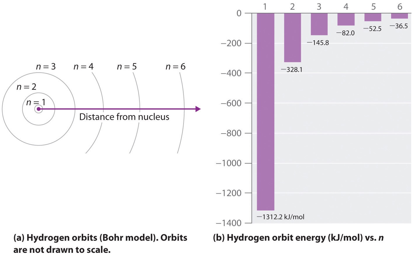
In this model, the regions of space are defined by their distance from the atom's nucleus. The distance correlates to the level of energy, n, holding the electron and the nucleus together and n = ∞ corresponds to the level where this energy is zero. In that level, the electron is unbound from the nucleus and the atom has been separated into a negatively charged (the electron) and a positively charged (the nucleus) ion. In this state the radius of the orbit is also infinite. The atom has been ionized.

Figure \(\PageIndex{2}\): The Bohr Model of the Hydrogen Atom (a) The distance of the orbit from the nucleus increases with increasing n. (b) The energy of the orbit becomes increasingly less negative with increasing n.

Niels Bohr (1885–1962)

During the Nazi occupation of Denmark in World War II, Bohr eventually escaped to the United States, where he became associated with the Atomic Energy Project.

In his final years, he devoted himself to the peaceful application of atomic physics and to resolving political problems arising from the development of atomic weapons.

As n decreases, the energy holding the electron and the nucleus together becomes increasingly negative, the radius of the orbit shrinks and more energy is needed to ionize the atom. The orbit with n = 1 is the lowest lying and most tightly bound (Figure \(\PageIndex{1}\)).

Figure \(\PageIndex{3}\): The Emission of Light by a Hydrogen Atom in an Excited State. (a) Light is emitted, represented by the wiggly arrow, when the electron undergoes a transition from an orbit with a higher value of n (at a higher energy) to an orbit with a lower value of n (at lower energy). (b) The Balmer series of emission lines is due to transitions from orbits with n ≥ 3 to the orbit with n = 2. The differences in energy between these levels corresponds to light in the visible portion of the electromagnetic spectrum.

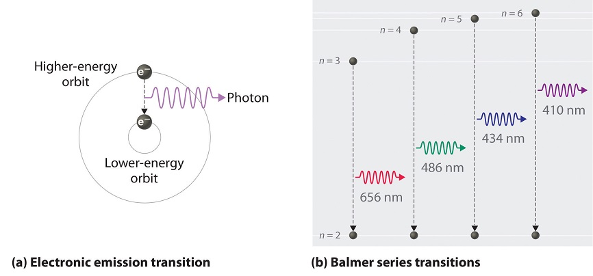
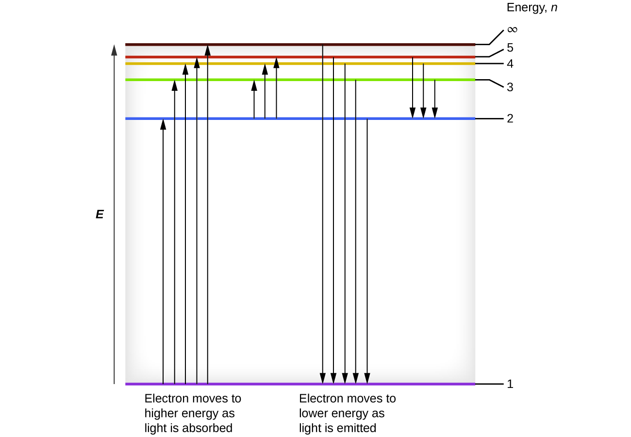
The negative sign in Equation \(\ref{6.3.2}\) indicates that the electron-nucleus pair is more tightly bound (i.e. at a lower potential energy) when they are near each other than when they are far apart. Because a hydrogen atom with its one electron in this orbit has the lowest possible energy, this is the ground state (the most stable arrangement of electrons for an element or a compound) for a hydrogen atom. As n increases, the radius of the orbit increases; the electron is farther from the proton, which results in a less stable arrangement with higher potential energy (Figure \(\PageIndex{2a}\)). A hydrogen atom with an electron in an orbit with n > 1 is therefore in an excited state, defined as any arrangement of electrons that is higher in energy than the ground state. When an atom in an excited state undergoes a transition to the ground state in a process called decay, it loses energy by emitting a photon whose energy corresponds to the difference in energy between the two states (Figure \(\PageIndex{4}\)).

Figure \(\PageIndex{4}\): The horizontal lines show the relative energy of orbits in the Bohr model of the hydrogen atom, and the vertical arrows depict the energy of photons absorbed (left) or emitted (right) as electrons move between these orbits.

So the difference in energy (\(ΔE\)) between any two orbits or energy levels is given by \( \Delta E=E_{n_{1}}-E_{n_{2}} \) where n₁ is the final orbit and n₂ the initial orbit. Substituting from Bohr’s equation (Equation \ref{6.3.3}) for each energy value gives

\[\begin{align*} \Delta E &=E_{final}-E_{initial} \\[4pt] &=-\dfrac{\Re hc}{n_{2}^{2}}-\left ( -\dfrac{\Re hc}{n_{1}^{2}} \right ) \\[4pt] &=-\Re hc\left ( \dfrac{1}{n_{2}^{2}} - \dfrac{1}{n_{1}^{2}}\right ) \label{6.3.4} \end{align*} \]

 

If \(n_2 > n_1\), the transition is from a higher energy state (larger-radius orbit) to a lower energy state (smaller-radius orbit), as shown by the dashed arrow in part (a) in Figure \(\PageIndex{3}\). Substituting \(hc/λ\) for \(ΔE\) gives

\[ \Delta E = \dfrac{hc}{\lambda }=-\Re hc\left ( \dfrac{1}{n_{2}^{2}} - \dfrac{1}{n_{1}^{2}}\right ) \label{6.3.5} \]

Canceling \(hc\) on both sides gives

\[ \dfrac{1}{\lambda }=-\Re \left ( \dfrac{1}{n_{2}^{2}} - \dfrac{1}{n_{1}^{2}}\right ) \label{6.3.6} \]

Except for the negative sign, this is the same equation that Rydberg obtained experimentally. The negative sign in Equations \(\ref{6.3.5}\) and \(\ref{6.3.6}\) indicates that energy is released as the electron moves from orbit \(n_2\) to orbit \(n_1\) because orbit \(n_2\) is at a higher energy than orbit \(n_1\). Bohr calculated the value of \(\Re\) from fundamental constants such as the charge and mass of the electron and Planck's constant and obtained a value of 1.0974 × 10⁷ m⁻¹, the same number Rydberg had obtained by analyzing the emission spectra.

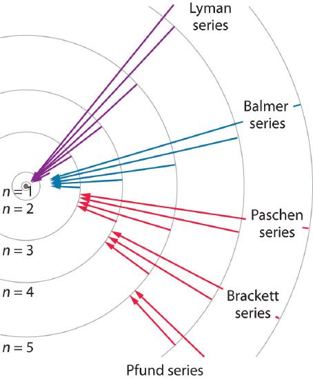
We can now understand the physical basis for the Balmer series of lines in the emission spectrum of hydrogen (\(\PageIndex{3b}\)); the lines in this series correspond to transitions from higher-energy orbits (n > 2) to the second orbit (n = 2). Thus the hydrogen atoms in the sample have absorbed energy from the electrical discharge and decayed from a higher-energy excited state (n > 2) to a lower-energy state (n = 2) by emitting a photon of electromagnetic radiation whose energy corresponds exactly to the difference in energy between the two states (Figure \(\PageIndex{3a}\)). The n = 3 to n = 2 transition gives rise to the line at 656 nm (red), the n = 4 to n = 2 transition to the line at 486 nm (green), the n = 5 to n = 2 transition to the line at 434 nm (blue), and the n = 6 to n = 2 transition to the line at 410 nm (violet). Because a sample of hydrogen contains a large number of atoms, the intensity of the various lines in a line spectrum depends on the number of atoms in each excited state. At the temperature in the gas discharge tube, more atoms are in the n = 3 than the n ≥ 4 levels. Consequently, the n = 3 to n = 2 transition is the most intense line, producing the characteristic red color of a hydrogen discharge (Figure \(\PageIndex{1a}\)). Other families of lines are produced by transitions from excited states with n > 1 to the orbit with n = 1 or to orbits with n ≥ 3. These transitions are shown schematically in Figure \(\PageIndex{4}\)

The Bohr Atom: https://youtu.be/GuFQEOzFOgA

Figure \(\PageIndex{5}\): Electron Transitions Responsible for the Various Series of Lines Observed in the Emission Spectrum of Hydrogen. The Lyman series of lines is due to transitions from higher-energy orbits to the lowest-energy orbit (n = 1); these transitions release a great deal of energy, corresponding to radiation in the ultraviolet portion of the electromagnetic spectrum. The Paschen, Brackett, and Pfund series of lines are due to transitions from higher-energy orbits to orbits with n = 3, 4, and 5, respectively; these transitions release substantially less energy, corresponding to infrared radiation. (Orbits are not drawn to scale.)

Using Atoms to Time

In contemporary applications, electron transitions are used in timekeeping that needs to be exact. Telecommunications systems, such as cell phones, depend on timing signals that are accurate to within a millionth of a second per day, as are the devices that control the US power grid. Global positioning system (GPS) signals must be accurate to within a billionth of a second per day, which is equivalent to gaining or losing no more than one second in 1,400,000 years. Quantifying time requires finding an event with an interval that repeats on a regular basis.

To achieve the accuracy required for modern purposes, physicists have turned to the atom. The current standard used to calibrate clocks is the cesium atom. Supercooled cesium atoms are placed in a vacuum chamber and bombarded with microwaves whose frequencies are carefully controlled. When the frequency is exactly right, the atoms absorb enough energy to undergo an electronic transition to a higher-energy state. Decay to a lower-energy state emits radiation. The microwave frequency is continually adjusted, serving as the clock’s pendulum.

In 1967, the second was defined as the duration of 9,192,631,770 oscillations of the resonant frequency of a cesium atom, called the cesium clock (more precisely this is the unperturbed ground state hyperfine transition frequency of the caesium-133 atom). Research is currently under way to develop the next generation of atomic clocks that promise to be even more accurate. Such devices would allow scientists to monitor vanishingly faint electromagnetic signals produced by nerve pathways in the brain and geologists to measure variations in gravitational fields, which cause fluctuations in time, that would aid in the discovery of oil or minerals.

Example \(\PageIndex{1}\): The Lyman Series

The so-called Lyman series of lines in the emission spectrum of hydrogen corresponds to transitions from various excited states to the n = 1 orbit. Calculate the wavelength of the lowest-energy line in the Lyman series to three significant figures. In what region of the electromagnetic spectrum does it occur?

Given: lowest-energy orbit in the Lyman series

Asked for: wavelength of the lowest-energy Lyman line and corresponding region of the spectrum

Strategy:

1. Substitute the appropriate values into Equation \ref{6.3.2} (the Rydberg equation) and solve for \(\lambda\).
2. Use Figure 2.2.1 to locate the region of the electromagnetic spectrum corresponding to the calculated wavelength.

Solution:

We can use the Rydberg equation to calculate the wavelength:

\[ \dfrac{1}{\lambda }=-\Re \left ( \dfrac{1}{n_{2}^{2}} - \dfrac{1}{n_{1}^{2}}\right ) \nonumber \]

A For the Lyman series, n₁ = 1. The lowest-energy line is due to a transition from the n = 2 to n = 1 orbit because they are the closest in energy.

\[ \dfrac{1}{\lambda }=-\Re \left ( \dfrac{1}{n_{2}^{2}} - \dfrac{1}{n_{1}^{2}}\right )=1.097\times m^{-1}\left ( \dfrac{1}{1}-\dfrac{1}{4} \right )=8.228 \times 10^{6}\; m^{-1} \nonumber \]

It turns out that spectroscopists (the people who study spectroscopy) use cm^-1 rather than m^-1 as a common unit. Wavelength is inversely proportional to energy but frequency is directly proportional as shown by Planck's formula, \(E=h u\).

Spectroscopists often talk about energy and frequency as equivalent. The cm^-1 unit is particularly convenient. The infrared range is roughly 200 - 5,000 cm^-1, the visible from 11,000 to 25.000 cm^-1 and the UV between 25,000 and 100,000 cm^-1. The units of cm^-1 are called wavenumbers, although people often verbalize it as inverse centimeters. We can convert the answer in part A to cm^-1.

\[ \widetilde{ u} =\dfrac{1}{\lambda }=8.228\times 10^{6}\cancel{m^{-1}}\left (\dfrac{\cancel{m}}{100\;cm} \right )=82,280\: cm^{-1} \nonumber \]

and

\[\lambda = 1.215 \times 10^{−7}\; m = 122\; nm \nonumber \]

This emission line is called Lyman alpha. It is the strongest atomic emission line from the sun and drives the chemistry of the upper atmosphere of all the planets, producing ions by stripping electrons from atoms and molecules. It is completely absorbed by oxygen in the upper stratosphere, dissociating O₂ molecules to O atoms which react with other O₂ molecules to form stratospheric ozone.

B This wavelength is in the ultraviolet region of the spectrum.

Exercise \(\PageIndex{1}\): The Pfund Series

The Pfund series of lines in the emission spectrum of hydrogen corresponds to transitions from higher excited states to the n = 5 orbit. Calculate the wavelength of the second line in the Pfund series to three significant figures. In which region of the spectrum does it lie?

Answer

4.65 × 10³ nm; infrared

Bohr’s model of the hydrogen atom gave an exact explanation for its observed emission spectrum. The following are his key contributions to our understanding of atomic structure:

Unfortunately, Bohr could not explain why the electron should be restricted to particular orbits. Also, despite a great deal of tinkering, such as assuming that orbits could be ellipses rather than circles, his model could not quantitatively explain the emission spectra of any element other than hydrogen (Figure \(\PageIndex{5}\)). In fact, Bohr’s model worked only for species that contained just one electron: H, He⁺, Li²⁺, and so forth. Scientists needed a fundamental change in their way of thinking about the electronic structure of atoms to advance beyond the Bohr model.

Figure \(\PageIndex{6}\): The atomic emission spectra for various elements. Each thin band in each spectrum corresponds to a single, unique transition between energy levels in an atom. Image from the Rochester Institute of Technology, CC BY-NC-SA 2.0.

The Energy States of the Hydrogen Atom

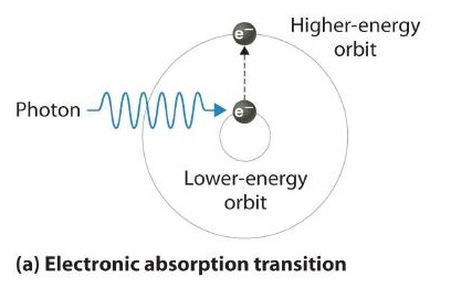
Thus far we have explicitly considered only the emission of light by atoms in excited states, which produces an emission spectrum (a spectrum produced by the emission of light by atoms in excited states). The converse, absorption of light by ground-state atoms to produce an excited state, can also occur, producing an absorption spectrum (a spectrum produced by the absorption of light by ground-state atoms).

When an atom emits light, it decays to a lower energy state; when an atom absorbs light, it is excited to a higher energy state.

If white light is passed through a sample of hydrogen, hydrogen atoms absorb energy as an electron is excited to higher energy levels (orbits with n ≥ 2). If the light that emerges is passed through a prism, it forms a continuous spectrum with black lines (corresponding to no light passing through the sample) at 656, 468, 434, and 410 nm. These wavelengths correspond to the n = 2 to n = 3, n = 2 to n = 4, n = 2 to n = 5, and n = 2 to n = 6 transitions. Any given element therefore has both a characteristic emission spectrum and a characteristic absorption spectrum, which are essentially complementary images.

Figure \(\PageIndex{7}\): Absorption and Emission Spectra. Absorption of light by a hydrogen atom. (a) When a hydrogen atom absorbs a photon of light, an electron is excited to an orbit that has a higher energy and larger value of n. (b) Images of the emission and absorption spectra of hydrogen are shown here. (CC BY-NC-SA 3.0; anonymous)

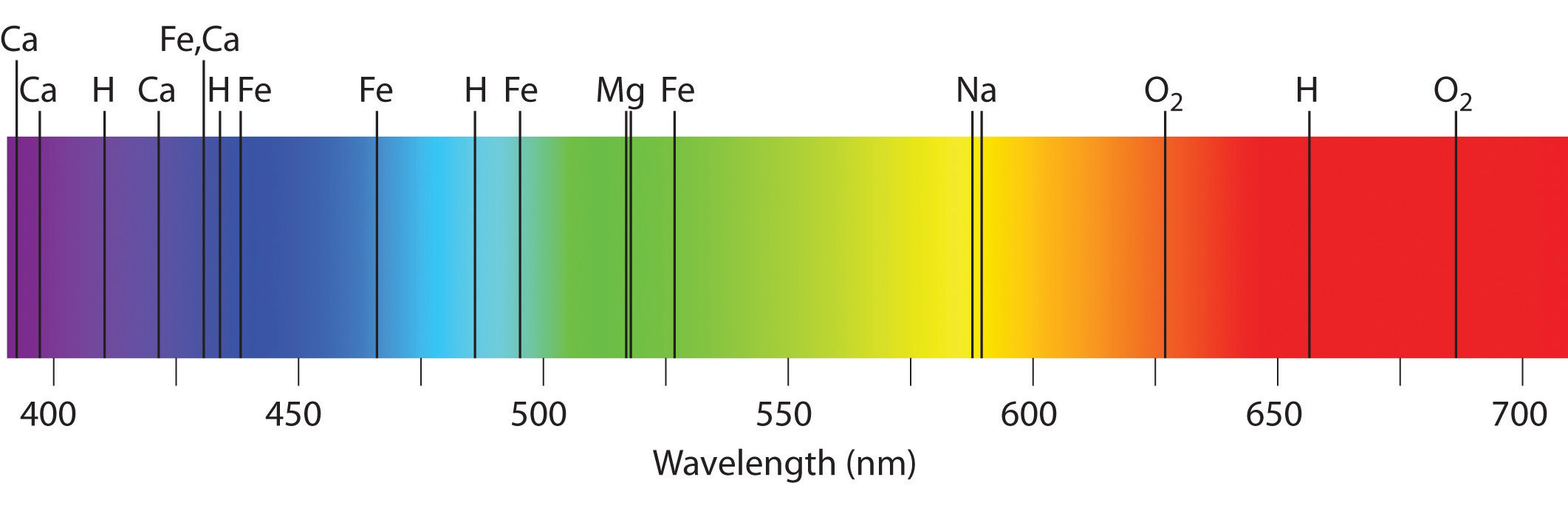
Emission and absorption spectra form the basis of spectroscopy, which uses spectra to provide information about the structure and the composition of a substance or an object. In particular, astronomers use emission and absorption spectra to determine the composition of stars and interstellar matter. As an example, consider the spectrum of sunlight shown in Figure \(\PageIndex{8}\) Because the sun is very hot, the light it emits is in the form of a continuous emission spectrum. Superimposed on it, however, is a series of dark lines due primarily to the absorption of specific frequencies of light by cooler atoms in the outer atmosphere of the sun. By comparing these lines with the spectra of elements measured on Earth, we now know that the sun contains large amounts of hydrogen, iron, and carbon, along with smaller amounts of other elements. During the solar eclipse of 1868, the French astronomer Pierre Janssen (1824–1907) observed a set of lines that did not match those of any known element. He suggested that they were due to the presence of a new element, which he named helium, from the Greek helios, meaning “sun.” Helium was finally discovered in uranium ores on Earth in 1895. Alpha particles are helium nuclei. Alpha particles emitted by the radioactive uranium pick up electrons from the rocks to form helium atoms.

Figure \(\PageIndex{8}\): The Visible Spectrum of Sunlight. The characteristic dark lines are mostly due to the absorption of light by elements that are present in the cooler outer part of the sun’s atmosphere; specific elements are indicated by the labels. The lines at 628 and 687 nm, however, are due to the absorption of light by oxygen molecules in Earth’s atmosphere. (CC BY-NC-SA 3.0; anonymous)

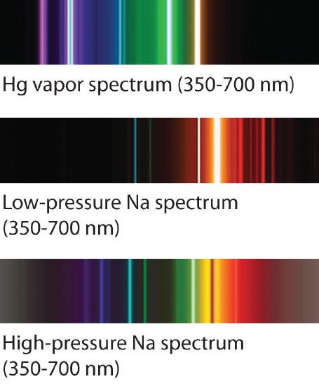
The familiar red color of neon signs used in advertising is due to the emission spectrum of neon shown in part (b) in Figure \(\PageIndex{5}\). Similarly, the blue and yellow colors of certain street lights are caused, respectively, by mercury and sodium discharges. In all these cases, an electrical discharge excites neutral atoms to a higher energy state, and light is emitted when the atoms decay to the ground state. In the case of mercury, most of the emission lines are below 450 nm, which produces a blue light (part (c) in Figure \(\PageIndex{6}\)). In the case of sodium, the most intense emission lines are at 589 nm, which produces an intense yellow light.

Figure \(\PageIndex{9}\): The emission spectra of sodium and mercury. Sodium and mercury spectra. Many street lights use bulbs that contain sodium or mercury vapor. Due to the very different emission spectra of these elements, they emit light of different colors. The lines in the sodium lamp are broadened by collisions. The dark line in the center of the high pressure sodium lamp where the low pressure lamp is strongest is cause by absorption of light in the cooler outer part of the lamp.

Summary

There is an intimate connection between the atomic structure of an atom and its spectral characteristics. Atoms of individual elements emit light at only specific wavelengths, producing a line spectrum rather than the continuous spectrum of all wavelengths produced by a hot object. Niels Bohr explained the line spectrum of the hydrogen atom by assuming that the electron moved in circular orbits and that orbits with only certain radii were allowed. Lines in the spectrum were due to transitions in which an electron moved from a higher-energy orbit with a larger radius to a lower-energy orbit with smaller radius. The orbit closest to the nucleus represented the ground state of the atom and was most stable; orbits farther away were higher-energy excited states. Transitions between these allowed orbits result in the absorption or emission of photons. When an electron moves from a higher-energy orbit to a more stable one, energy is emitted in the form of a photon. To move an electron from a stable orbit to a more excited one, a photon of energy must be absorbed. These produce for each element, respectively, an absorption spectrum, which has dark lines, and an emission spectrum, which has bright lines in the same position. Using the Bohr model, we can calculate the energy of an electron and the radius of its orbit in any one-electron system. Bohr’s model revolutionized the understanding of the atom but could not explain the spectra of atoms heavier than hydrogen.

Glossary

Bohr’s model of the hydrogen atom

structural model in which an electron moves around the nucleus only in circular orbits, each with a specific allowed radius; the orbiting electron does not normally emit electromagnetic radiation, but does so when changing from one orbit to another.

absorption spectrum

The dark narrow lines produced when the light passing through an excited element is measured

emission spectrum

The bright narrow lines produced when the light emitted from an excited element is passed through a prism

excited state

state having an energy greater than the ground-state energy

ground state

state in which the electrons in an atom, ion, or molecule have the lowest energy possible

line spectrum

A few narrow lines of particular wavelengths observed rather than a continuous range of wavelengths

quantum number

integer number having only specific allowed values and used to characterize the arrangement of electrons in an atom

Contributors and Attributions

• Modified by Joshua Halpern (Howard University)