
2.10: Colorimetric pH measurement
- Page ID
- 435380
\( \newcommand{\vecs}[1]{\overset { \scriptstyle \rightharpoonup} {\mathbf{#1}} } \)
\( \newcommand{\vecd}[1]{\overset{-\!-\!\rightharpoonup}{\vphantom{a}\smash {#1}}} \)
\( \newcommand{\id}{\mathrm{id}}\) \( \newcommand{\Span}{\mathrm{span}}\)
( \newcommand{\kernel}{\mathrm{null}\,}\) \( \newcommand{\range}{\mathrm{range}\,}\)
\( \newcommand{\RealPart}{\mathrm{Re}}\) \( \newcommand{\ImaginaryPart}{\mathrm{Im}}\)
\( \newcommand{\Argument}{\mathrm{Arg}}\) \( \newcommand{\norm}[1]{\| #1 \|}\)
\( \newcommand{\inner}[2]{\langle #1, #2 \rangle}\)
\( \newcommand{\Span}{\mathrm{span}}\)
\( \newcommand{\id}{\mathrm{id}}\)
\( \newcommand{\Span}{\mathrm{span}}\)
\( \newcommand{\kernel}{\mathrm{null}\,}\)
\( \newcommand{\range}{\mathrm{range}\,}\)
\( \newcommand{\RealPart}{\mathrm{Re}}\)
\( \newcommand{\ImaginaryPart}{\mathrm{Im}}\)
\( \newcommand{\Argument}{\mathrm{Arg}}\)
\( \newcommand{\norm}[1]{\| #1 \|}\)
\( \newcommand{\inner}[2]{\langle #1, #2 \rangle}\)
\( \newcommand{\Span}{\mathrm{span}}\) \( \newcommand{\AA}{\unicode[.8,0]{x212B}}\)
\( \newcommand{\vectorA}[1]{\vec{#1}} % arrow\)
\( \newcommand{\vectorAt}[1]{\vec{\text{#1}}} % arrow\)
\( \newcommand{\vectorB}[1]{\overset { \scriptstyle \rightharpoonup} {\mathbf{#1}} } \)
\( \newcommand{\vectorC}[1]{\textbf{#1}} \)
\( \newcommand{\vectorD}[1]{\overrightarrow{#1}} \)
\( \newcommand{\vectorDt}[1]{\overrightarrow{\text{#1}}} \)
\( \newcommand{\vectE}[1]{\overset{-\!-\!\rightharpoonup}{\vphantom{a}\smash{\mathbf {#1}}}} \)
\( \newcommand{\vecs}[1]{\overset { \scriptstyle \rightharpoonup} {\mathbf{#1}} } \)
\( \newcommand{\vecd}[1]{\overset{-\!-\!\rightharpoonup}{\vphantom{a}\smash {#1}}} \)
\(\newcommand{\avec}{\mathbf a}\) \(\newcommand{\bvec}{\mathbf b}\) \(\newcommand{\cvec}{\mathbf c}\) \(\newcommand{\dvec}{\mathbf d}\) \(\newcommand{\dtil}{\widetilde{\mathbf d}}\) \(\newcommand{\evec}{\mathbf e}\) \(\newcommand{\fvec}{\mathbf f}\) \(\newcommand{\nvec}{\mathbf n}\) \(\newcommand{\pvec}{\mathbf p}\) \(\newcommand{\qvec}{\mathbf q}\) \(\newcommand{\svec}{\mathbf s}\) \(\newcommand{\tvec}{\mathbf t}\) \(\newcommand{\uvec}{\mathbf u}\) \(\newcommand{\vvec}{\mathbf v}\) \(\newcommand{\wvec}{\mathbf w}\) \(\newcommand{\xvec}{\mathbf x}\) \(\newcommand{\yvec}{\mathbf y}\) \(\newcommand{\zvec}{\mathbf z}\) \(\newcommand{\rvec}{\mathbf r}\) \(\newcommand{\mvec}{\mathbf m}\) \(\newcommand{\zerovec}{\mathbf 0}\) \(\newcommand{\onevec}{\mathbf 1}\) \(\newcommand{\real}{\mathbb R}\) \(\newcommand{\twovec}[2]{\left[\begin{array}{r}#1 \\ #2 \end{array}\right]}\) \(\newcommand{\ctwovec}[2]{\left[\begin{array}{c}#1 \\ #2 \end{array}\right]}\) \(\newcommand{\threevec}[3]{\left[\begin{array}{r}#1 \\ #2 \\ #3 \end{array}\right]}\) \(\newcommand{\cthreevec}[3]{\left[\begin{array}{c}#1 \\ #2 \\ #3 \end{array}\right]}\) \(\newcommand{\fourvec}[4]{\left[\begin{array}{r}#1 \\ #2 \\ #3 \\ #4 \end{array}\right]}\) \(\newcommand{\cfourvec}[4]{\left[\begin{array}{c}#1 \\ #2 \\ #3 \\ #4 \end{array}\right]}\) \(\newcommand{\fivevec}[5]{\left[\begin{array}{r}#1 \\ #2 \\ #3 \\ #4 \\ #5 \\ \end{array}\right]}\) \(\newcommand{\cfivevec}[5]{\left[\begin{array}{c}#1 \\ #2 \\ #3 \\ #4 \\ #5 \\ \end{array}\right]}\) \(\newcommand{\mattwo}[4]{\left[\begin{array}{rr}#1 \amp #2 \\ #3 \amp #4 \\ \end{array}\right]}\) \(\newcommand{\laspan}[1]{\text{Span}\{#1\}}\) \(\newcommand{\bcal}{\cal B}\) \(\newcommand{\ccal}{\cal C}\) \(\newcommand{\scal}{\cal S}\) \(\newcommand{\wcal}{\cal W}\) \(\newcommand{\ecal}{\cal E}\) \(\newcommand{\coords}[2]{\left\{#1\right\}_{#2}}\) \(\newcommand{\gray}[1]{\color{gray}{#1}}\) \(\newcommand{\lgray}[1]{\color{lightgray}{#1}}\) \(\newcommand{\rank}{\operatorname{rank}}\) \(\newcommand{\row}{\text{Row}}\) \(\newcommand{\col}{\text{Col}}\) \(\renewcommand{\row}{\text{Row}}\) \(\newcommand{\nul}{\text{Nul}}\) \(\newcommand{\var}{\text{Var}}\) \(\newcommand{\corr}{\text{corr}}\) \(\newcommand{\len}[1]{\left|#1\right|}\) \(\newcommand{\bbar}{\overline{\bvec}}\) \(\newcommand{\bhat}{\widehat{\bvec}}\) \(\newcommand{\bperp}{\bvec^\perp}\) \(\newcommand{\xhat}{\widehat{\xvec}}\) \(\newcommand{\vhat}{\widehat{\vvec}}\) \(\newcommand{\uhat}{\widehat{\uvec}}\) \(\newcommand{\what}{\widehat{\wvec}}\) \(\newcommand{\Sighat}{\widehat{\Sigma}}\) \(\newcommand{\lt}{<}\) \(\newcommand{\gt}{>}\) \(\newcommand{\amp}{&}\) \(\definecolor{fillinmathshade}{gray}{0.9}\)Your task today is to estimate the pH-values of six solutions using an indicator, and then getting a better estimate by measuring the absorbance of the indicator at two different wavelengths. This dual-wavelength method is used commercially, for example in Pulse Oxymeters to measure oxygen saturation of hemoglobin in our blood, shining light through our fingertip. Similar techniques are also used to measure concentrations or pH in living cells.
The reason we are using two wavelengths is to figure out the hue of the color irrespective of its intensity. Said in another way, the two-wavelength measurement will give the same result for different concentrations of the indicator, as long as the ratio of protonated to deprotonated is the same.
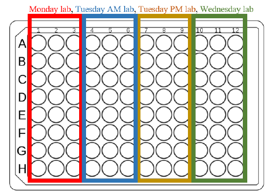
For this experiment, we will be storing and measuring solutions in a 96-well plate. These are used in situations where you have a lot of samples of similar type, and are designed for automation. Each group will have their own plate, but it is used in the other sections too, so please only use the designated well:
Tasks (you are working in pairs)
There are two data sheets; one of you will use the first, and one of you will use the second. Use the first data sheet for tasks 1-8. Then, switch recorder and use the second data sheet for tasks 9 and 10. Finally, record your critical evaluation of the experiment on the back side of your data sheets.
- Using a transfer pipette, place approximately 250 µL of each buffer you are testing in two adjacent wells in the microplate(e.g. first column and second column, rows A-F). Make sure not to contaminate (cross-contaminate) the buffers, as they will be used by other lab sections as well.
- Place one drop of universal indicator into the six solutions in the first column. Determine the pH range of your solution (by comparing with the standards), and choose whether to work with phenol red (color change at about pH 7) or methyl red (color change at about pH 5 to 5.5). Communicate that choice to your instructor.
- Place one drop of the chosen indicator into the buffers in the second column.
- The exact pKa of the indicator will depend on the temperature, the solvent, the ionic strength (the concentration and charge of ions present), so we will measure it using a standard. There are four standards available (pH 5 or pH 8, low or high ionic strength). Choose the one most appropriate and consult your instructor. Place one drop of the chosen indicator into three empty wells (e.g. row H), and add 250 µL each of your pH standard solution of choice.
- Place the microplate in the reader, measure the absorbance at two wavelengths (540 nm, 405 nm, already set) and record the absorbance. You will have to use the menu to switch the display between the two wavelengths (if you have a way of taking two pictures, that is the most reliable and fast method).
- Using the calibration curve for the indicator (there is one for methyl red and a different one for phenol red), estimate what fraction is protonated and what fraction is deprotonated for each of the nine samples. To do this, first calculate (A540 – A405) / (A540 + A405), then read off the percentage of deprotonated indicator. The percentage of protonated indicator is 100% minus that value.
- Estimate the pKa of your indicator from the three solutions with known pH. You will use the Henderson-Hasselbalch relationship with the pKa as an unknown (see sample calculation 1). Use the average of the three values as your best estimate of the pKa.
- Now, again using the Henderson-Hasselbalch relationship, calculate the pH of the six buffers with unknown pH (see sample calculation 2). The pKa in the formula refers to that of the indicator, and [HA]/[A-] to the ratio of protonated to deprotonated indicator.
Switch to the other data sheet. - Add 100 µL of 50 mM HCl to each of the solutions made in task 3 (second column, the ones with methyl or phenol red). Visually, which changed color the most?
- Measure the absorption and calculate the pH. Which solution had the largest change in pH? What factors determine how much the pH changes? Do your measured pH shifts match your prediction?
- Find the other group working on the same solutions. Compare your results to theirs and to the measurements made with a pH electrode last week.