
2.9: Making a buffer with three components
- Page ID
- 435381
\( \newcommand{\vecs}[1]{\overset { \scriptstyle \rightharpoonup} {\mathbf{#1}} } \)
\( \newcommand{\vecd}[1]{\overset{-\!-\!\rightharpoonup}{\vphantom{a}\smash {#1}}} \)
\( \newcommand{\id}{\mathrm{id}}\) \( \newcommand{\Span}{\mathrm{span}}\)
( \newcommand{\kernel}{\mathrm{null}\,}\) \( \newcommand{\range}{\mathrm{range}\,}\)
\( \newcommand{\RealPart}{\mathrm{Re}}\) \( \newcommand{\ImaginaryPart}{\mathrm{Im}}\)
\( \newcommand{\Argument}{\mathrm{Arg}}\) \( \newcommand{\norm}[1]{\| #1 \|}\)
\( \newcommand{\inner}[2]{\langle #1, #2 \rangle}\)
\( \newcommand{\Span}{\mathrm{span}}\)
\( \newcommand{\id}{\mathrm{id}}\)
\( \newcommand{\Span}{\mathrm{span}}\)
\( \newcommand{\kernel}{\mathrm{null}\,}\)
\( \newcommand{\range}{\mathrm{range}\,}\)
\( \newcommand{\RealPart}{\mathrm{Re}}\)
\( \newcommand{\ImaginaryPart}{\mathrm{Im}}\)
\( \newcommand{\Argument}{\mathrm{Arg}}\)
\( \newcommand{\norm}[1]{\| #1 \|}\)
\( \newcommand{\inner}[2]{\langle #1, #2 \rangle}\)
\( \newcommand{\Span}{\mathrm{span}}\) \( \newcommand{\AA}{\unicode[.8,0]{x212B}}\)
\( \newcommand{\vectorA}[1]{\vec{#1}} % arrow\)
\( \newcommand{\vectorAt}[1]{\vec{\text{#1}}} % arrow\)
\( \newcommand{\vectorB}[1]{\overset { \scriptstyle \rightharpoonup} {\mathbf{#1}} } \)
\( \newcommand{\vectorC}[1]{\textbf{#1}} \)
\( \newcommand{\vectorD}[1]{\overrightarrow{#1}} \)
\( \newcommand{\vectorDt}[1]{\overrightarrow{\text{#1}}} \)
\( \newcommand{\vectE}[1]{\overset{-\!-\!\rightharpoonup}{\vphantom{a}\smash{\mathbf {#1}}}} \)
\( \newcommand{\vecs}[1]{\overset { \scriptstyle \rightharpoonup} {\mathbf{#1}} } \)
\( \newcommand{\vecd}[1]{\overset{-\!-\!\rightharpoonup}{\vphantom{a}\smash {#1}}} \)
\(\newcommand{\avec}{\mathbf a}\) \(\newcommand{\bvec}{\mathbf b}\) \(\newcommand{\cvec}{\mathbf c}\) \(\newcommand{\dvec}{\mathbf d}\) \(\newcommand{\dtil}{\widetilde{\mathbf d}}\) \(\newcommand{\evec}{\mathbf e}\) \(\newcommand{\fvec}{\mathbf f}\) \(\newcommand{\nvec}{\mathbf n}\) \(\newcommand{\pvec}{\mathbf p}\) \(\newcommand{\qvec}{\mathbf q}\) \(\newcommand{\svec}{\mathbf s}\) \(\newcommand{\tvec}{\mathbf t}\) \(\newcommand{\uvec}{\mathbf u}\) \(\newcommand{\vvec}{\mathbf v}\) \(\newcommand{\wvec}{\mathbf w}\) \(\newcommand{\xvec}{\mathbf x}\) \(\newcommand{\yvec}{\mathbf y}\) \(\newcommand{\zvec}{\mathbf z}\) \(\newcommand{\rvec}{\mathbf r}\) \(\newcommand{\mvec}{\mathbf m}\) \(\newcommand{\zerovec}{\mathbf 0}\) \(\newcommand{\onevec}{\mathbf 1}\) \(\newcommand{\real}{\mathbb R}\) \(\newcommand{\twovec}[2]{\left[\begin{array}{r}#1 \\ #2 \end{array}\right]}\) \(\newcommand{\ctwovec}[2]{\left[\begin{array}{c}#1 \\ #2 \end{array}\right]}\) \(\newcommand{\threevec}[3]{\left[\begin{array}{r}#1 \\ #2 \\ #3 \end{array}\right]}\) \(\newcommand{\cthreevec}[3]{\left[\begin{array}{c}#1 \\ #2 \\ #3 \end{array}\right]}\) \(\newcommand{\fourvec}[4]{\left[\begin{array}{r}#1 \\ #2 \\ #3 \\ #4 \end{array}\right]}\) \(\newcommand{\cfourvec}[4]{\left[\begin{array}{c}#1 \\ #2 \\ #3 \\ #4 \end{array}\right]}\) \(\newcommand{\fivevec}[5]{\left[\begin{array}{r}#1 \\ #2 \\ #3 \\ #4 \\ #5 \\ \end{array}\right]}\) \(\newcommand{\cfivevec}[5]{\left[\begin{array}{c}#1 \\ #2 \\ #3 \\ #4 \\ #5 \\ \end{array}\right]}\) \(\newcommand{\mattwo}[4]{\left[\begin{array}{rr}#1 \amp #2 \\ #3 \amp #4 \\ \end{array}\right]}\) \(\newcommand{\laspan}[1]{\text{Span}\{#1\}}\) \(\newcommand{\bcal}{\cal B}\) \(\newcommand{\ccal}{\cal C}\) \(\newcommand{\scal}{\cal S}\) \(\newcommand{\wcal}{\cal W}\) \(\newcommand{\ecal}{\cal E}\) \(\newcommand{\coords}[2]{\left\{#1\right\}_{#2}}\) \(\newcommand{\gray}[1]{\color{gray}{#1}}\) \(\newcommand{\lgray}[1]{\color{lightgray}{#1}}\) \(\newcommand{\rank}{\operatorname{rank}}\) \(\newcommand{\row}{\text{Row}}\) \(\newcommand{\col}{\text{Col}}\) \(\renewcommand{\row}{\text{Row}}\) \(\newcommand{\nul}{\text{Nul}}\) \(\newcommand{\var}{\text{Var}}\) \(\newcommand{\corr}{\text{corr}}\) \(\newcommand{\len}[1]{\left|#1\right|}\) \(\newcommand{\bbar}{\overline{\bvec}}\) \(\newcommand{\bhat}{\widehat{\bvec}}\) \(\newcommand{\bperp}{\bvec^\perp}\) \(\newcommand{\xhat}{\widehat{\xvec}}\) \(\newcommand{\vhat}{\widehat{\vvec}}\) \(\newcommand{\uhat}{\widehat{\uvec}}\) \(\newcommand{\what}{\widehat{\wvec}}\) \(\newcommand{\Sighat}{\widehat{\Sigma}}\) \(\newcommand{\lt}{<}\) \(\newcommand{\gt}{>}\) \(\newcommand{\amp}{&}\) \(\definecolor{fillinmathshade}{gray}{0.9}\)Your job today is to make a buffered solution. We are not giving you the procedure, just the final concentrations in the solution. You will receive a "recipe card" such as the one below.
|
Solution B5 Make 50 mL of a buffer containing: · 50 mM sodium citrate, · 20 mM HBr · 100 mM KCl |
Please work carefully and check your calculations. Other students (in this and other sections) will use this buffer next week for a colorimetric lab.
Research labs and industrial labs typically have a variety of solutions on hand to do their daily work. Often, these are made by one person and used by many. When hiring new people to work in the lab, one crucial question is whether they are able to make solutions that others can use with confidence.
This lab has two parts. In the first part, you are responsible for figuring out a recipe for your solution and for making it. In the second part, you team up to characterize your solutions, and to submit a solution you feel is closest to the specifications.
You have the following materials available:
- Pure sodium acetate trihydrate (NaCH3COO·3 H2O, powder, molar mass is ~136 g/mol)
- Pure sodium phosphate, monobasic monohydrate
- (NaH2PO4·H2O, powder, molar mass is ~138 g/mol)
- Solution of hydrochloric acid, HCl, concentration is 200 mM (or value on the bottle)
- Solution of sodium hydroxide, NaOH, concentration is 200 mM (or value on the bottle)
- Solution of sodium chloride, NaCl, concentration is 2.00 M
- Solution of sodium chloride, NaCl, concentration is 0.200 M
Part one: individual tasks
Record your calculations and measurements in the data sheet.
- Formulate a recipe to make your buffered solution. You will weigh out a certain mass of your buffer substance, add strong acid or base (this will adjust the pH), add sodium chloride and water. Choose which NaCl stock solution you will use to minimize volume errors.
- Make the buffer, using your recipe and checking off steps as you go. If there are any unexpected issues, take notes. Also, record the exact mass you used (it is fine if it is a couple of milligrams different from your recipe).
- Calculate the estimated pH of your solution after looking up the relevant pKa value.
Tasks (working together)
- Find the other individual(s) working on the same solution. Compare the recipes you used and the pH values you calculated. While the recipes might differ a bit, the calculated pH should be the same.
- Measure the pH of your two solutions. You have measured pH values during lab last week. Use the same procedure, making sure the electrode is rinsed between uses. If you missed the lab, ask for a demonstration before you use the pH meter. The pH is sensitive to concentrations of acids and bases added (as well as which acid or base you added). The same recipe should always give the same or a similar pH. For comparisons, it is best to use the same pH meter (they might be calibrated slightly differently).
- Measure the conductivity of your two solutions: The conductivity is influenced by which ions are present at which concentration. Identical solutions should have the same conductivity. For the solutions we are making today, the biggest influence on conductivity is the concentration of sodium chloride. Inconsistencies in the sodium chloride concentration would show as a large difference in conductivity but only a small difference in pH (because NaCl is neither an acid nor a base). We are using an analog instrument that is a bit quirky. The following instructions will make more sense when you are at the instrument or after watching the video (QR code below).

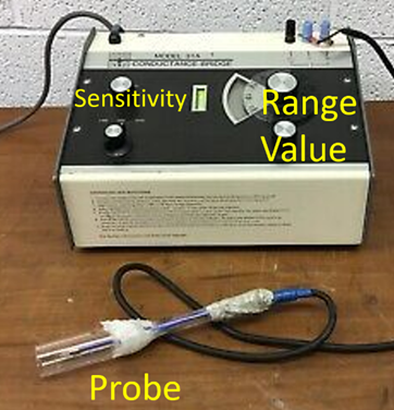
For the conductivity measurement, make sure the probe and the provided 50 mL tube are rinsed with water before they come in contact with you solution. Transfer your solution into the 50 mL tube and insert the probe. For an accurate measurement, the probe has to be submerged past the line. Then, choose the appropriate measurement interval using the range dial while the sensitivity knob is turned all the way counterclockwise. Finally, increase the sensitivity, adjust the value dial to maximize the gap in the display, and read off the result on both dials. Don’t forget to retrieve your solution once you are done. There are two sample solutions provided along with the measurements if you need to troubleshoot. - Enter the data in the data table in your report, and discuss how different the measurements are for the different solutions. Are the differences within the range you expected? If not, what might have happened?
- Decide what you want to save for next week. You can either submit a mixture of your solutions (this would average out random errors) or decide to submit a single solution and dump the rest. If you discover that all solutions made had some “fatal flaw”, you can also make another solution together and submit that.
- Place your buffer in a 50 mL screw cap tube. Make a label, indicating the concentrations of all components, the data and your (first) names, and tape it on the tube. Then, put your solution in the provided Styrofoam rack in the hood.