1.2: The First Law of Thermodynamics

Systems can undergo a change of state from some initial state to a final state accompanied by a change in the system’s energy. In this chapter, we analyze two types of energy: heat and work. This leads to a presentation of the first law of thermodynamics that deals with the conservation of energy, stating that any changes in the total internal energy of the system must be due to exchanges of either heat or work with the surroundings. Emphasis is placed on ideal gases because their equation of state is known. We also introduce an important property of a material, the heat capacity, that allows us to calculate the change in temperature as a function of heat. Finally, the concept of enthalpy is introduced that plays an important role in biochemical reactions.

Learning Objectives

• Be able to explain and give some examples of state properties.
• Be able to define heat and work and understand heat and work are types of energy.
• Understand that heat and work are path-dependent (not state properties).
• Understand that energy is conserved: changes in the total internal energy must be due to either heat flow into/out of the system in relation to the surroundings or work being done on/ being performed by the system in relation to the surroundings.
• Be able to calculate the change in energy, enthalpy, work and heat exchange for the compression/expansion of an ideal gas and generalize these observations to other systems.

State properties and the internal Energy (U)

In Chapter I.1, we introduced the concept of an equation of state that relates state properties (also called state variables or state functions). State properties describe the thermodynamic state of the system in terms of quantifiable observables such as temperature, pressure, volume, and number of moles for an ideal gas.

An important feature of state properties is that they are independent of the system’s history. In other words, if the system is changed from some initial state to a final state, the corresponding change in any state function does not depend on the path taken from the initial to final state or on any intermediate states. An example of a state property is the total internal energy of the system, which we will give the symbol \(\bf{U}\). The total internal energy includes the translational, rotational, vibrational, electronic, and nuclear energies of all the particles, as well as the energy due to intermolecular interactions.

Figure I.2.A shows a schematic energy diagram of changing the system from some initial state A into some final state B.

Figure I.2.A The change in internal energy (U) in going from some initial state A to some final state B does not depend on the process of going from A to B but only on the difference in energy between A and B.

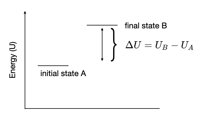
Notice that the overall change in energy, \(\Delta U\) does not depend on how the system was change from \(A \rightarrow B\). For state variables we write the change if energy

\[\Delta U = U_{f}-U_{i} \]

As an example, consider a piston containing an ideal gas as shown in Figure I.2.B:

Figure I.2.B: A gas at an initial temperature, pressure, and volume has an initial energy given by U_init. Expanding the piston an infinitesimal amount dV, the infinitesimal change in energy is dU. After expansion of the gas the system is in a new state with a different temperature, volume, pressure. The final energy is U_final.

Since the molecules do not interact, the total internal energy depends only on the kinetic energy of all the gas molecules, which is related to the temperature. We now expand the piston through a series of infinitesimal steps such that the temperature of the gas changes as the volume increases. At each infinitesimal step, the infinitesimal change in the internal energy is \(dU\). Summing over all the infinitesimal steps gives the total change in internal energy as

\[\int_{U_i}^{U_f} dU = U_{f}-U_{i} = \Delta U\label{EQ:deltaU}\]

Mathematically, \(\bf{dU}\) is an exact differential (see Appendix), meaning that integration from an initial state to a final state is independent of the path. For any state property \(dz\), the differential is exact, and we can write:

\[\int_{z_i}^{z_f} dz = \Delta z\label{EQ:exactdiff}\]

Equation \ref{EQ:exactdiff} will serve as a definition of a state property since all state properties are exact differentials because they are independent of the path.

Work

We have seen how the total internal energy is a state property of system. At this point, we might ask ourselves what would be an example of a quantity that is not a state property? One such example would be the work done by the system in going from an initial to a final state. Work is the physical activity directed towards the production of accomplishing something. Work can be performed on the system by the surroundings, or work can be done by the system on the surroundings; however, work is not an intrinsic property of the system itself and is not a state property. The amount of work performed will depend on the path taken to change the state from some initial state to some final state. As an example, we can consider a hiker walking in the Sehome Arboretum. Figure I.2.C shows the situation of a hiker starting at some initial position A and reaching the final position B by two different paths. Because these paths are different, the hikers will have performed a different amount of work in traveling from point A to point B, depending on the path taken.

Figure I.2.C: Two hikers in the Sehome Arboretum travel from the same initial point A to the same final point B, but they travel by different paths. Because the paths differ, the hikers will have performed a different amount of work in traversing from A to B.

In classical mechanics the work is defined as the force times the distance. For an infinitesimal displacement \(\bf{dx}\) the work is

\[\delta w = F\cdot dx\label{EQ:mechanicalwork}\]

where \(\bf{F}\) is the applied force.

Note

Note: The quantity \(\delta w\) denotes an infinitesimal increment of work. It should be noted that work is not a state function, meaning that the differential is inexact and Equation \ref{EQ:exactdiff} cannot be applied. Instead, we write the total work over a path taken from some initial state to some final state as:

\[w = \int_{path} \delta w \]

Because the differential \(\delta w\) is inexact, the integral over different paths with the same end points will be different.

In thermodynamics we generalize this concept of work to consider different types of work summarized in Table I.2.i:

Table I.2.i: Various types of work and their mathematical expressions

Types of work	\(\delta w\)	Generic force, displacement

mechanical work	F · dx	F is the force, dx is the distance
Surface work	γ · dA	γ is the surface tension, dA is the change in area
Electrical work	φ · dQ	φ is the electric potential difference, dQ is the electric charge
Gravitational work	mg · dh	mg is the gravitational acceleration, dh is the change in height
Stretching work	τ · dL	τ is the tension, dL is the change in length
Expansion (compression)	P · dV	P is the pressure, dV is the change in volume

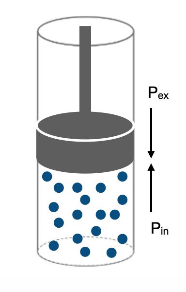
We will mainly focus our attention on the expansion (compression) type work of work (sometimes called PV-work) of a gas in a cylinder. Figure I.2.D shows the situation of a gas in a cylinder with a piston with some opposing, external pressure, \(\bf{P_{ex}}\), acting on the gas.

Figure I.2.D: A gas in a cylinder with a piston. An external pressure pushing down on the piston acts to oppose the expansion of the gas.

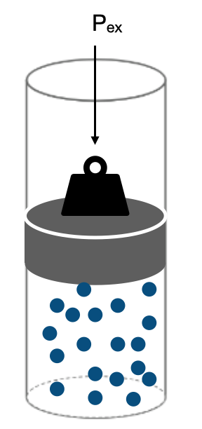
Because the external pressure is pushing against the gas (the direction of the force is pointing down on the piston), we define the work of expansion as:

\[\delta w \equiv -P_{ex} \cdot dV\label{EQ:workdef}\]

where \(\bf{\delta w}\) is some infinitesimal amount of work and \(\bf{dV}\) is an infinitesimal change in the volume due to expansion or compression of the piston. Equation \ref{EQ:workdef} is the definition of the work of expansion/compression of a gas. Let’s look at some examples for how to calculate the work for a gas in a cylinder.

Example 1: Expansion of a gas against a constant pressure

As our first example, we consider the expansion of a gas against a constant pressure. The situation is shown in Figure I.2.E. Initially, two masses oppose the piston. Removal of one of the masses, causes the gas in the cylinder to expand against the constant pressure due to the remaining mass from an initial volume \(\bf{V_i}\) to a final volume \(\bf{V_f}\).

Figure I.2.E: Expansion of a gas against a constant pressure. A gas is held at an initial volume V_i by two masses on a piston. Upon removal of one of the masses, the gas expands to a new volume V_f against a constant pressure P_ext.

The total work performed by the gas can be calculated by integrating Equation \ref{EQ:workdef}

\[w = -\int_{V_i}^{V_f} P_{ext} \cdot dV\label{EQ:work_irrev1}\]

Because the external applied pressure in this case is constant, it can be taken out of the integral to give:

\[\begin{eqnarray}w &=& -P_{ext} \int_{V_i}^{V_f} dV \nonumber \\[4pt] &=& -P_{ext} \Delta V\label{EQ:work_irrev2}\end{eqnarray}\]

where \(\Delta V=(V_f – V_i)\). Notice that in the last line we have used the fact that the volume is a state variable so that \(\Delta V= \int dV\).

Key Result: The work performed during the expansion of a gas against a constant external pressure is \( w = -P_{ext} \cdot \Delta V\)

See Practice Problem 1.

Example 2: Free expansion of a gas against a vacuum.

We now consider a slightly different situation when a gas is allowed to freely expand into a vacuum. The situation is illustrated in Figure I.2.F. A gas is compressed to a volume V_i by a piston that is held in placed by a mass, and a vacuum is created by removal of air from the space above the piston. When the mass is removed, the gas will freely expand against the vacuum to fill the cylinder to a final volume of V_f.

Figure I.2.F: Expansion of a gas into a vacuum. In the cylinder on the left, an applied pressure is used to compress a gas, and a vacuum is created in the space above the piston. When the weight is removed (middle cylinder), the compressed gas will expand from an initial volume V_i against the vacuum until it occupies the available space (right cylinder) with final volume V_f.

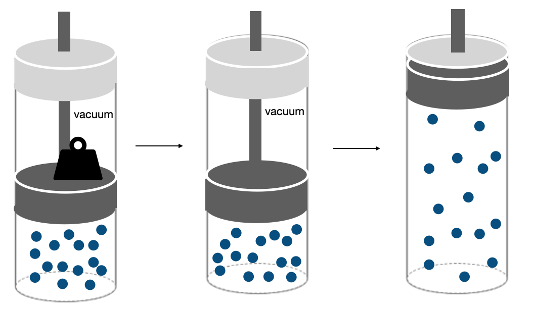
We can again use Equation \ref{EQ:workdef} to obtain:

\[w = -P_{ext} \cdot \Delta V\]

However, here we note that the external pressure \(P_{ext}=0\) because the gas is expanding into a vacuum. Thus, the work performed by the expansion is \(w=0\).

Key Result: There is no work performed in the free expansion of a gas against a vacuum. \(w=0\).

See Practice Problems 2 and 3.

Work is not a state property

Notice that in the first example the work performed in expanding the gas was \(w=-P_{ext}\cdot \Delta V\), but in the second example, expanding the gas to the same final volume against a vacuum resulted in no work being performed. Thus, we see that the amount of work being performed depends on the path taken and hence work is not a state property.

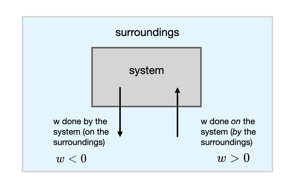
Note: In this book we adopt the convention that work being performed on the system by the surroundings is positive. This means that work being performed by the system on the surroundings will be negative by convention. Work being done on the system by the surrounding is shown on the left panel of Figure I.2.G with an arrow showing the direction of work pointing from the surroundings to the system. The right panel of Figure I.2.G shows the situation of work being performed by the system with an arrow pointing form the system to the surroundings. For the situation on the right, the work will have a negative sign.

Figure I.2.G: Sign convention for work. Work performed by the system on the surrounding is depicted by an arrow pointing form the system to the surroundings and has a negative sign by convention. Work performed on the system (by the surroundings) is depicted by an arrow pointing from the surroundings into the system and is positive by convention.

Heat

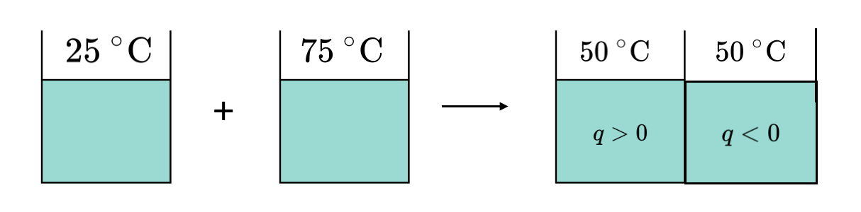
Heat is another type of energy that can flow across the system boundary causing the system to change its state. As an example we can consider the situation shown in Figure 1.2.H of two liquids: one at 25 °C and one at 75 °C. If the two containers are brought into thermal contact, heat will flow out of the hotter (75 °C) liquid into the cooler (25 °C) liquid until thermal equilibrium is reached and both liquids reach the same final temperature.

Figure I.2.H: When two systems at different temperature are brought into thermal contact, heat will flow from the hotter system into the colder system until the two systems are at thermal equilibrium.

Heat is not a state property

Just like work, heat is not a state property, and the amount of heat flow into or out of the system depends on the path taken from the initial state to the final state. We will use the symbol \(q\) to represent heat.

Note: In this book we adopt the same sign convention that we used for work. Heat being absorbed by the system from the surroundings will be defined as positive and represented with an arrow pointing from the surroundings to the system to indicate the direction of heat flow. On the other hand, heat given off by the system into the surroundings will have a negative sign and will be depicted with an arrow pointing from the system into the surroundings as shown in Figure I.2.I

Figure I.2.I Sign convention for heat. Heat flowing out of the system into the surroundings (exothermic) is depicted by an arrow pointing form the system to the surroundings and has a negative sign by convention. Heat flowing into the system from the surroundings (endothermic) is depicted by an arrow pointing from the surroundings into the system and is positive by convention.

The Zeroth Law of Thermodynamics

The concept that heat flows from hot to cold establishes what is known as the zeroth law of thermodynamics. The zeroth law states that if system A is in thermal equilibrium with system B, and system B is in thermal equilibrium with system C, then system A must also be in thermal equilibrium with systems C. Figure I.2.J summarizes the zeroth law of thermodynamics.

Figure I.2.J: The Zeroth Law of Thermodynamics establishes that if two systems (A and B) are in thermal equilibrium with each other and another system (C) is brought into thermal equilibrium with one of the systems (B), then C is also in thermal equilibrium with system A.

Although conceptually simple, the zeroth law is important because it formally establishes temperature as a well-defined quantity.

First Law of Thermodynamics

Having defined heat and work as types of energy, we are now in a position to state the first law of thermodynamics. The first law states that the change in energy (\(\Delta U\)) of a system is equal to the sum of the work done on the system (\(w\)) and heat (\(q\)) put into the system. Mathematically, we can express the first law as:

\[\Delta U = q + w\label{EQ:firstlaw}\]

We see from Equation \ref{EQ:firstlaw} that the first law of thermodynamics is a statement about the conservation of energy. In order for the energy of the system to change, energy must be transferred to/from the surroundings in the form of either heat or work.

For dealing with infinitesimal changes of energy (\(dU\)) the first law can be written in differential form:

\[dU = \delta q + \delta w\label{EQ:firstlaw_diff}\]

Reversible vs. Irreversible Processes

Both Example 1 and Example 2 above are examples of an irreversible process, meaning that the expansion against a constant pressure or against a vacuum occurs spontaneously in one direction, but the reverse process does not occur spontaneously. This directionality of spontaneous change results from the fact that the system is not maintained at equilibrium during the expansion. When the gas is expanding, the pressure inside is not equal to the external applied pressure causing a net force to push the gas molecules into the larger volume.

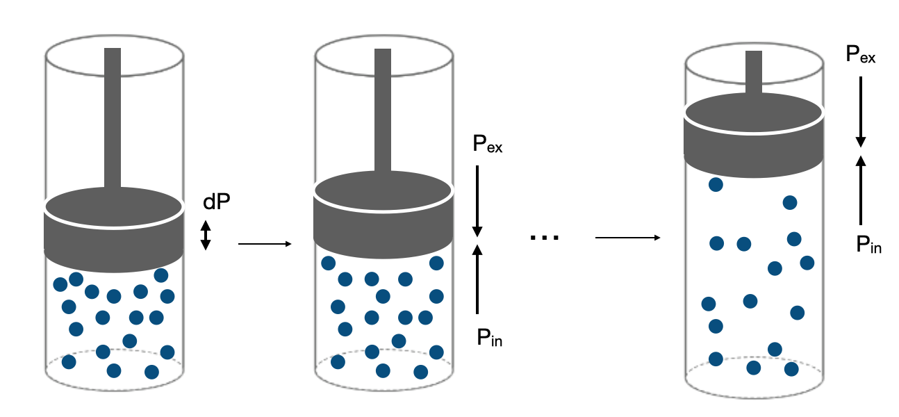
Imagine the situation shown in Figure I.2.K where the internal pressure of the gas is equal to the external pressure applied by the piston. Figure I.2.K represents the system at equilibrium.

Figure I.2.K: A gas in a cylinder at equilibrium with the surroundings. At equilibrium the pressure exerted by the gas on the piston (P_in) is equal and opposite to the pressure exerted by the surroundings on the piston (P_ex).

We could now consider expanding the gas through a series of infinitesimal steps where equilibrium is maintained throughout the expansion by adjusting the external pressure so that it is always equal to the internal pressure of the gas. Note that in this case the external applied pressure will not be constant since it is adjusted to maintain equilibrium at each step. The situation is illustrated in Figure I.2.L. At each infinitesimal step, there is no net force pushing the gas to change volume in any one direction so the process is said to be reversible.

Figure I.2.L: Reversible expansion of a gas. A gas in a cylinder initially at volume V_i is slowly expanded to a final volume V_f such that the internal pressure P_in remains equal and opposite to the external pressure P_ex at each infinitesimal step. During a reversible process, quasi-equilibrium is maintained throughout.

A reversible process is a process which is at equilibrium at each infinitesimal step. Because work depends on the path (not a state property), the amount of work performed (and thus also the amount of heat flow) will depend on if the process occurs reversibly or irreversibly. As an example we will consider the reversible expansion of a gas.

Example 3: Isothermal Reversible Expansion of a Gas

Consider the isothermal reversible expansion of a gas. The situation is similar to the situation illustrated in Figure I.2.L. The gas is initially at a volume V_i and is expanded reversibly to a final volume of V_f while maintaining a constant temperature. Because the processes is reversible, the external pressure (\(\bf{P_{ext}}\)) is always equal to the internal pressure of the gas (\(\bf{P_{in}}\)) which can both be replaced by the variable \(P=P_{in}=P_{ext}\). The work is again calculated by integrating Equation \ref{EQ:workdef}:

\[w = -\int_{V_i}^{V_f} P \cdot dV\label{EQ:work_rev}\]

Note that in this case, we cannot take the variable \(\bf{P}\) outside of the integral because the pressure is not constant but depends on the volume during the expansion. In order to proceed, we need to know how the pressure \(\bf{P}\) depends on the volume \(\bf{V}\). For an ideal gas, we know the relation from the ideal gas equation of state:

\[P=\frac{nRT}{V}\label{EQ:Pin}\]

Substituting this into Equation \ref{EQ:work_rev} gives:

\[w = -\int_{V_i}^{V_f} \frac{nRT}{V} \cdot dV\label{EQ:w_rev2}\]

We can now use the fact that \(\bf{n}\) (constant number of moles), \(\bf{R}\), and \(\bf{T}\) (isothermal = constant temperature) are constants and can be pulled out of the integral so that the integrand only depends on the volume:

\[\begin{eqnarray}w &=& -nRT \int_{V_i}^{V_f} \frac{dV}{V} \nonumber \\[4pt] &=& -nRT \ln \left(\frac{V_f}{V_i}\right)\label{EQ:w_rev3}\end{eqnarray}\]

Note

We have used the integral: \( \int \frac{1}{x} dx = \ln x +C \)

Key Result: For the reversible isothermal expansion of a gas, the work performed is \(w=-nRT \ln \left(\frac{V_f}{V_i}\right)\)

See Practice Problems 4 and 5

Maximum Work Theorem

A comparison of Equation \ref{EQ:w_rev3} with the result above from Equation \ref{EQ:work_irrev2} shows that the amount of work performed is different if the process is performed reversibly than if the process is performed irreversibly. Figure I.2.M shows a plot of the Pressure vs. the Volume for the two different expansions. A plot of P vs. V is called a PV-diagram and the work performed is the area under the curve. Notice that the work performed (area under the curve) is greater for the reversible expansion than the work performed for the irreversible expansion. It turns out that for any reversible process, the amount of work performed is maximized as compared to the equivalent irreversible processes. This principle is called the maximum work theorem.

Key result: The maximum work theorem states that for all processes leading from a specified initial state to some specified final state, the work performed is a maximum for a reversible process.

Figure I.2.M Left: The situation described in Example 1 of the irreversible expansion of a gas against a constant pressure. Right: The situation described in Example 3 of the reversible expansion of a gas. The area under the curve between the initial state and final state is the magnitude of the work performed by the piston. Note that that area under the curve is always greater in the reversible process.

The Heat Capacity

A useful property of a system is the heat capacity. The heat capacity is the amount of energy (heat) required to raise the temperature of a material by some infinitesimal amount \(dT\).

\[\delta q = C\cdot dT\label{EQ:heatcapacity}\]

Equation \ref{EQ:heatcapacity} says that the amount of heat transferred to the systems (\(\delta q\)) is proportional to the change in temperature (\(dT\)) and the proportionality factor is the heat capacity of the material. How much the temperature rises in a material as it is heated depends on:

• the amount of heat delivered (q)
• the amount of substance present
• the chemical nature and physical state of the material
• the conditions under which the energy is added

Integrating both sides of Equation \ref{EQ:heatcapacity} from an initial temperature \(\bf{T_i}\) to a final temperature \(\bf{T_f}\) gives:

\[q = \int_{T_i}^{T_f} C \cdot dT\label{EQ:heatcapacity2}\]

In general, the heat capacities \(\bf{C}\) also depend on the temperature. However, for an ideal gas, the heat capacity is independent of temperature and can be taken out of the integral to give:

\[\begin{eqnarray}q &=& C \int_{T_i}^{T_f} dT \nonumber \\[4pt] q &=& C \Delta T\label{EQ:heatcapacity3}\end{eqnarray}\]

where \(\Delta T=T_f – T_i\) and we have used the fact that temperature is a state property.

For a gas, the heat capacity depends on whether the gas undergoes a change of state at constant volume conditions (isochoric) or at constant pressure conditions (isobaric).

We denote the heat capacity at constant volume as \(C_v\) and the heat capacity at constant pressure as \(C_p\). At constant volume we have:

\[\delta q_v = C_v\cdot dT\label{EQ:heatcapacity_V}\]

and at constant pressure we have:

\[\delta q_p = C_p\cdot dT\label{EQ:heatcapacity_P}\]

where the subscript indicates whether we are under conditions of constant volume or pressure. Rearranging Equation \ref{EQ:heatcapacity_V} and Equation \ref{EQ:heatcapacity_P} we see that the heat capacity is given by:

\[C_v = \left(\frac{\partial q}{\partial T}\right)_V\label{EQ:heatcapacity_V2}\]

and at constant pressure we have:

\[C_p = \left(\frac{\partial q}{\partial T}\right)_P\label{EQ:heatcapacity_P2}\]

The heat capacities \(C_p\) and \(C_v\) are the slope of the curve of heat vs. temperature.

Enthalpy

We saw above that work and heat depend on the path taken from an initial state to a final state. Let’s consider in more detail the reversible expansion/compression of a gas in a cylinder under the conditions of constant pressure (isobaric). From the first law of the thermodynamics we can write the change of energy as:

\[\begin{eqnarray}dU &=& \delta q_p + \delta w \nonumber \\[4pt] dU &=& \delta q_p - P\cdot dV\label{EQ:enthalpy1}\end{eqnarray}\]

where the subscript on \(\delta q_p\) indicates we are under conditions of constant pressure (isobaric) and we have used the fact that the reversible work is \(\delta w = -P\cdot dV\). Rearranging Equation \ref{EQ:enthalpy1} for \(\delta q_p\) we have:

\[\begin{eqnarray}\delta q_p &=& dU + PdV \nonumber \\[4pt] \delta q_p &=& d(U+PV)\label{EQ:enthalpy2}\end{eqnarray}\]

where the second line is true because the pressure \(\bf{P}\) is constant. We now introduce a new quantity called the enthalpy that gets the symbol \(\bf{H}\) that is defined as the energy + PV:

\[H = U + PV\label{EQ:Hdef}\]

Equation \ref{EQ:Hdef} is the definition of the enthalpy. Substituting Equation \ref{EQ:Hdef} into Equation \ref{EQ:enthalpy2} gives:

\[\delta q_p = dH\label{EQ:Hdef2}\]

or, upon integrating both sides:

\[q_p = \Delta H\label{EQ:Hdef3}\]

From Equation \ref{EQ:Hdef2} and Equation \ref{EQ:Hdef3}, we see that the change in enthalpy of the system is equal to the amount of heat gained by the system under the conditions of constant pressure.

Key result: Enthalpy is defined as: \(H = U+PV\)

Key result: The change in enthalpy of the system is equal to the heat gained by the system at constant pressure: \(q_p = \Delta H\)

Note

Note: Although heat is not a state property and thus depends on the path, the enthalpy \(H\) is a state property and so the change of enthalpy \(\Delta H\) will be independent of the path taken.

Heat Capacity Revisited

Constant Pressure

Recall that the heat capacity for a gas depends on if the conditions are isobaric (constant P) or isochoric (constant V). At constant pressure, we copy the expression from Equation \ref{EQ:heatcapacity_P} above:

\[\delta q_p = C_p\cdot dT \nonumber \]

We have also shown that the heat gained at constant pressure is equivalent to the change in enthalpy \(\bf{dH}\) (Equation \ref{EQ:Hdef2}). Substituting Equation \ref{EQ:Hdef2} into Equation \ref{EQ:heatcapacity_P} gives:

\[dH = C_p\cdot dT\label{EQ:heatcapacity_PH1}\]

or, rearranging in terms of \(C_p\):

\[C_p = \left(\frac{\partial H}{\partial T}\right)_P\label{EQ:heatcapacity_PH2}\]

Equation \ref{EQ:heatcapacity_PH2} shows that the slope of the enthalpy \(\bf{H}\) with respect to the temperature \(\bf{T}\) at constant pressure is the heat capacity \(\bf{C_p}\).

Constant Volume

At constant volume, we copy the expression from Equation \ref{EQ:heatcapacity_V} above:

\[\delta q_v = C_v\cdot dT\label{EQ:heatcapacity_Vnew}\]

From the first law of thermodynamics we have the change in energy \(\bf{dU}\) is given by: \( dU = \delta q_v -PdV \) where the subscript \(\bf{\delta q_v}\) indicates we are at constant volume conditions. Since the volume is constant, there is no work being performed since \(\bf{dV=0}\). At constant volume conditions we can write:

\[dU = \delta q_v\label{EQ:dU_constv}\]

since all the change in energy at constant volume is due to heat flow (no work). Substituting Equation \ref{EQ:dU_constv} into Equation \ref{EQ:heatcapacity_Vnew} gives:

\[dU = C_v\cdot dT\label{EQ:heatcapacity_VU1}\]

or, rearranging in terms of \(\bf{C_v}\):

\[C_v = \left(\frac{\partial U}{\partial T}\right)_V\label{EQ:heatcapacity_VU2}\]

Equation \ref{EQ:heatcapacity_VU2} shows that the slope of the energy \(\bf{U}\) with respect to the temperature \(\bf{T}\) at constant volume is the heat capacity \(\bf{C_v}\).

Relation between \(C_v\) and \(C_p\) for an ideal gas

To relate \(\bf{C_v}\) and \(\bf{C_p}\) for an ideal gas, we begin with the definition of the enthalpy: \( H = U +PV.\) Recall that for an ideal gas, \(PV=nRT.\) Substituting the ideal gas law into the definition of the enthalpy gives:

\[H=U + nRT\label{EQ:enthalpy_idealgas}\]

Note that because we have use the ideal gas law, Equation \ref{EQ:enthalpy_idealgas} only applies to an ideal gas. Taking \(\bf{n}\) and \(\bf{R}\) to be constants, we can write the differential form of Equation \ref{EQ:enthalpy_idealgas} as:

\[dH = dU + nR dT\label{EQ:enthalpy_ideal_gas2}\]

Substituting Equation \ref{EQ:heatcapacity_VU1} and Equation \ref{EQ:heatcapacity_PH1} into Equation \ref{EQ:enthalpy_ideal_gas2} and dividing out the \(dT\) gives:

\[C_p = C_v + nR\label{EQ:ideal_gasCp_Cv}\]

Equation \ref{EQ:ideal_gasCp_Cv} relates the heat capacity at constant pressure \(\bf{C_p}\) and the heat capacity at constant volume \(\bf{C_v}\) for an ideal gas.

Key result: For an ideal gas the heat capacity at constant pressure \(C_p\) and the heat capacity at constant volume \(C_v\) are related by \( C_p = C_v + nR\)

See Practice Problem 6

Examples

Example \(\PageIndex{1}\)

One mole of an ideal gas in a cylinder is initially held at 12 atm of pressure and 298 K. Calculate the work done by a piston if the gas is expanded against a constant external pressure of 1.0 atm while the temperature is kept constant at 298 K.

Solution

For the expansion of an ideal gas at constant external pressure the work is given by Equation \ref{EQ:work_irrev2}

\( w = -P_{ext} \cdot \Delta V\)

First, we use PV=nRT to find the initial and final volumes of the gas:

\( V_i = \frac{1 \ \text{mole} \ \times \ \ 0.08206 \ \text{L atm K}^{-1} \ \text{mol}^{-1} \ \times \ 298 \ \text{K}}{12 \ \text{atm}} \)

\(V_i =2.038 \ \text{L} \)

Note that the final pressure inside the cylinder is equal to the external pressure of 1.0 atm:

\( V_f = \frac{1 \ \text{mole} \ \times \ \ 0.08206 \ \text{L atm K}^{-1} \ \text{mol}^{-1} \ \times \ 298 \ \text{K}}{1 \ \text{atm}} \)

\(V_f =24.45 \ \text{L} \)

This gives the total work as:

\( w = -1.0 \ \text{atm} (24.45 \ \text{L} - 2.038 \ \text{L})\)

\( w = -22.4 \ \text{L atm}\)

\( w = -22.4 \ \text{L atm} \times \ \frac{101.325 \ \text{J}}{1 \ \text{L atm}} = -2270 \ \text{Joules} \)

Notice in the final step we convert L atm to Joules, which is the more conventional energy units. Also notice that the sign of the work is negative by our convention because the system is doing work on the surroundings (expansion).

Example \(\PageIndex{2}\)

During the reversible isothermal compression of 3.0 moles of an ideal gas at T=291 K, the pressure changes from 3.0 atm to 5.0 atm. Calculate the work done.

Solution

We use the fact that for the reversible isothermal expansion of a gas, the work performed is \(w=-nRT \ln \left(\frac{V_f}{V_i}\right)\) (See Equation \ref{EQ:w_rev3}).

For an ideal gas at constant number of moles and constant temperature:

\(\frac{V_f}{V_i} = \frac{P_i}{P_f}\)

So the work (for an isothermal process) can be expressed in terms of the pressure as:

\(w=-nRT \ln \left(\frac{P_i}{P_f}\right)\)

\(w=-3.0 \ \text{moles} \ \times \ \ 8.314 \ \text{J K}^{-1} \ \text{mol}^{-1} \ \times \ 291 \ \text{K} \ \ln \left(\frac{3.0}{5.0}\right)\)

\(w=3707.6 \ \text{Joules} \)

Note that the work is positive by our convention since the surroundings is doing work on the system (compression).

Example \(\PageIndex{3}\)

The molar heat capacity at constant volume of a monatomic idea gas is 3/2 R. How much heat must be added to raise the temperature of 2.0 moles of an ideal gas by 10 °C?

Solution

We use the fact that the heat at constant volume is given by Equation \ref{EQ:heatcapacity_V}:

\(\delta q_v = C_v \cdot dT\)

Integrating both sides gives:

\(q_v = C_v \Delta T\)

Inserting the definition of the molar heat capacity \(\bar{C_v} = C_v/n \) into our expression for the heat gives:

\(q_v = n \bar{C_v} \Delta T\)

where n is the number of moles. Now we solve for the heat:

\(q_v = 2.0 \ \text{moles} \ \times \ \frac{3}{2} \ \times 8.314 \ \text{J K}^{-1} \ \text{mol}^{-1} \ \times \ 10 \ \text{K} \)

\(q_v = 249.42 \ \text{Joules}\)

Practice Problems

Problem 1. Consider an experiment where a gas is compressed isothermally (constant temperature) from an initial pressure of 1.0 atm and a volume of 3.0 L to a final pressure of 4.0 atm and a volume of 1.0 L. The temperature remains constant at 20.0 °C. Calculate the work done if the compression is performed in a single step against a constant external pressure of 4.0 atm. (Report your answer in Joules).

Problem 2. You are traveling in a space ship whose cabin volume is 10.0 m³ . The air inside the cabin is maintained at 1 atm and 298 K, suitable for human space travel. Suddenly, the cabin springs a leak, allowing 1.8 moles of gas to escape into the vacuum before you are able to repair the damage. Calculate a) q, b) w, and c) \(\Delta U\) for this process, assuming that the walls of the cabin are perfect insulators (adiabatic).

Problem 3. Calculate the work done when 50.0 g of iron reacts with hydrochloric acid:

Fe (s) + 2 HCl (aq) → FeCl₂ (aq) + H₂ (g)

assuming the reaction takes place in a) a closed vessel of fixed volume, and b) an open beaker at 25 °C. (The atomic mass of iron is 55.85 g/mol)

Problem 4. In Example 3 of the main text an expression was derived for the reversible isothermal expansion of an ideal gas. Now consider the reversible expansion of a gas under isobaric (constant P) conditions. Show that for the reversible isobaric expansion of an ideal gas the work is

\[ w = -n R \Delta T \]

(Hint: start with the definition of the work of expansion as \(dw = -P_{ex}\cdot dV\).)

Problem 5. Derive an expression for \(\Delta H\), \(\Delta U\), \(w\), and \(q\) for the reversible expansion of an ideal gas under the following conditions: a) isobaric (Hint: see Problem 4), b) isochoric (constant V), c) isothermal (Hint: see Example 3), d) adiabatic (no heat flow, Hint: q=0).

Problem 6. The molar heat capacity for liquid methanol is \(\bar{C_v}=68.624\) J K\(^{-1}\) mol\(^{-1}\). The density of methanol is 0.792 g/mL. How much heat is released when 50 mL of liquid methanol is cooled from 60 °C to 10 °C? If the process is performed in an open container, what is the change in enthalpy \(\Delta H\)? (Hint: \(\bar{C_v} \approx \bar{C_p}\) for a liquid).