1.1: Thermodynamic Variables and Equations of State

Classical thermodynamics provides a conceptual framework from which we can understand the behavior of molecular systems in the biological sciences at a quantitative level. This chapter introduces some of the concepts relating to properties of a system and its surroundings that we will need to study classical thermodynamics. Applications to biological systems will be presented in later chapters. In this chapter, we will focus on how the macroscopic properties of a system are related to and depend on the properties of the constituent atoms and molecules. As an example we will discuss the ideal-gas equation, its range of validity, and how it can be extended to real gases or fluids of interacting molecules.

Learning Objectives

• Build a precise vocabulary of thermodynamic definitions before applying them to biochemical systems.
• Understand state variables and how they are mathematically related in an equation of state.
• Be able to manipulate the ideal gas equation of state.
• Understand how real gases deviate from ideality and how real gases and fluids can be modeled by the virial equation of state, which is an expression for the pressure of a gas as a polynomial in the density.

Basic Definitions

We begin our discussion of biochemical thermodynamics with some definitions that will allow us to make general statements about how energy is exchanged and converted into various forms.

A system is any part of the universe that is of interest to us. This might be the Sun-Earth-Moon system, a human lung, fruit fly, a single bacteria cell, or a beaker on a bench top. Some example systems are shown in Figure I.1.A:

Figure I.1.A: Some systems of varying complexity include the sun-earth-moon system, a human lung, a fruit fly, a single bacteria cell, or a beaker

Everything else in the universe that is not part of the system is called the surroundings. The system + the surroundings constitutes the universe.

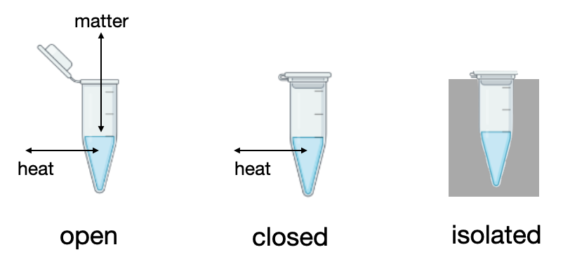
We can classify systems into 3 types: open systems, closed systems, or isolated systems. An open system is able to exchange both matter and heat with the surroundings. A closed system cannot exchange matter with the surroundings but can exchange heat with the surroundings. An isolated system cannot exchange any heat or any matter with surroundings. These three types of systems are depicted in Figure I.1.B:

Figure I.1.B: An open system can exchange both matter and heat with the surroundings. A closed system cannot exchange matter with the surroundings but can exchange heat. An isolated system cannot exchange heat or matter with the surroundings.

The branch of science called thermodynamics is interested in the relationships between properties of a system and how properties change as the system changes state. A property is any mathematically quantifiable parameter of the system. Some properties could include the pressure, the temperature, the density, the index of refraction, etc ….

We can distinguish between two types of properties: intensive and extensive. Intensive properties are independent of the quantity (amount of matter) being measured. Some intensive properties include the density, pressure, and temperature. On the other hand, Extensive properties depend on the quantity (amount) being measured. Some extensive properties are the mass, the volume, and the number of moles.

Intensive properties can be constructed as the ratio between two extensive properties. For example the density is

\[\text{density} = \frac{\text{mass}}{\text{volume}}\label{EQ:densitydef}\]

Notice that both mass and volume are extensive (depend on the amount), but the density (the ratio of the mass over volume) is intensive.

Similarly, the pressure is defined as

\[\text{pressure} = \frac{\text{force}}{\text{area}}\label{EQ:pressdef}\]

The SI units of pressure is the Pascal (Pa) and 1 Pa = 1 N\(\cdot\) m\(^{-2}\) = 1 kg\(\cdot\)m\(^{-1}\cdot\) s\(^{-2}\) = 1 J\(\cdot\) m\(^{-3}\). Table I.1.i relates some common units of pressure.

Table I.1.i: Some common units of pressure

1 Pa = 1 N m^-2

1 bar = 100 kPa (10^5Pa)

1 atm = 101.32 kPa

1 torr (mm Hg) = 1/760 atm

Note: Energy by itself (measured in Joules or calories) is an extensive property. Often, we report energies as a molar ratio in units of J/mol or cal/mol which is an intensive property.

A common way to define an intensive property is to define the molar quantity by dividing some extensive variable by the number of moles. For example, the molar volume is defined as:

\[\bar{V} = \frac{V}{n}\label{EQ:molarV}\]

Here \(\bf{n}\) is the number of moles and \(\bf{\bar{V}}\) is called the molar volume and is an intensive quantity.

Temperature is another important thermodynamic parameter that will be defined in serval ways throughout this text. For now, we will define the temperature as the measure of the motion of the atoms within the system. This definition of temperature implies that the “thermodynamic” temperature is measured in Kelvin, because the Kelvin scale is the absolute temperature scale. In the limit that T=0 K (absolute zero), the motion of the atoms approaches zero. We can convert between temperature in Kelvin and Celsius scales using the relation:

\[T (\text{in Kelvins})=T (\text{in }^{\circ}C) + 273.15\label{EQ:Temp}\]

Caution

Note: Absolute temperatures (in K) must be used in thermodynamic calculations.

See Practice Problems 1 and 2.

Thermodynamic Equations of State

An equation of state is a mathematical expression that fully describes the thermodynamic state of the system in terms of a set of physical properties. The most familiar example is the ideal gas law:

\[PV=nRT\label{EQ:idealgas}\]

or, introducing the molar volume (Equation \ref{EQ:molarV}):

\[P\bar{V} = RT\]

where \(\bf{P}\) is the pressure, \(\bf{V}\) is the volume, \(\bf{n}\) is the number of moles, \(\bf{T}\) is the temperature. \(\bf{R}\) is the gas constant given in Table I.1.ii. Equation \ref{EQ:idealgas} is known as the ideal gas equation of state. The ideal gas equation of state (PV=nRT) allows us to see how the properties of an ideal gas are related.

Table I.1.ii: Common units for the ideal gas constant R.

R = 8.314 J K^-1 mol^-1= 0.08206 L atm K^-1 mol^-1 L atm = 101.34 J

The ideal gas equation of state will be a useful model for us to work with as we derive thermodynamic relationships because it is intuitive and algebraically easy to manipulate. At this point, it is worthwhile to make some comments concerning the ideal gas equation of state:

1. The ideal gas equation of state can be derived from first principles (kinetic theory of gases).
2. At sufficiently high temperature and low pressure, all gases fit the ideal gas law.
3. Assumptions made in the ideal gas law:
   • The gas molecules themselves occupy no volume.
   • There are no attractive or repulsive forces between gas molecules.
   • All collisions are perfectly elastic.

See Practice Problems 3 and 4.

Because of these assumptions, we expect all real gases to deviate from ideal behavior. To quantify this we define the compressibility factor, Z, as

\[Z=\frac{P\bar{V}}{RT}\label{EQ:compress}\]

Notice from Equation \ref{EQ:idealgas} that for an ideal gas, \(Z=1.\) All real gases will deviate from this ideal behavior. Figure I.1.C shows the compressibility factor \(Z\) as a function of pressure for N₂ gas at different temperatures. A perfect ideal gas would have \(Z=1\) for all pressures and temperatures. For N₂ gas we see that at sufficiently low pressure \(Z \rightarrow 1\) and that at higher temperature (purple curve), the gas behalves more like an ideal gas (dotted line).

Figure I.1.C: Compressibility factor of nitrogen gas as a function of pressure for different temperatures. The ideal gas limit is shown by the dotted line at Z=1.

In order to derive an equation of state for a non-ideal gas, we can consider a series expansion of the compressibility factor, \(\bf{Z}\), in powers of the inverse molar volume, \(\bf{1/\bar{V}}\):

\[Z = 1 + \frac{B_2}{\bar{V}}+\frac{B_3}{\bar{V}^2}+\frac{B_4}{\bar{V}^3}+…\label{EQ:Virial}\]

Equation \ref{EQ:Virial} is called the virial equation of state, and \(\bf{B_2}\) is called the second virial coefficient, \(\bf{B_3}\) is called the third virial coefficient, etc…. The virial coefficients (\(B_2\), \(B_3\), …) are typically fit to experimental data and are temperature dependent. Notice that for a perfect ideal gas, the second and higher virial coefficients are all zero. The virial equation of state works well to describe any gas, but has the drawback of needing the virial coefficients from fitting to experimental data.

For gases that exhibit small deviations from ideal gas behavior, we can truncate Equation \ref{EQ:Virial} to include just the second virial coefficient:

\[Z \approx 1 + \frac{B_2}{\bar{V}}\label{EQ:Virial2}\]

The second viral coefficient, \(\bf{B_2}\) is related to the interactions between atoms described by a potential energy function \(U(r)\), where \(r\) is the distance between atom pairs. For a dilute system of non-polar molecules, the relationship between the second virial coefficient and the potential energy is

\[B_{2} = N_A \frac{1}{2} \int_0^{\infty} \left[1-e^{-U(r)/k_BT} \right] 4\pi r^2 dr\label{EQ:Virial3}\]

where \(\bf{N_A}\) is Avogadro’s number, \(\bf{k_B}\) is Boltzmann’s constant, and \(\bf{T}\) is the temperature. In most cases, we cannot analytically solve the integral in Equation \ref{EQ:Virial3}. Note that in the absence of interactions, \(U(r)=0\), then from Equation \ref{EQ:Virial3}, \(B_2=0\) and the gas behaves like an ideal gas as we would expect for non-interacting gas molecules.

See Practice Problems 5-7.

Osmotic Pressure and Osmotic Virial Coefficients

In dealing with solutions (either solutions of small molecule solutes or macromolecules in solution), an important colligative property is the osmotic pressure. The osmotic pressure is given by the symbol \( \Pi \) and is different from the pressure of a gas (P) because it does not arise from collisions of molecules against the wall of a container. The osmotic pressure is a hydrostatic pressure that arises when solvent molecules pass through a semipermeable membrane to the more concentrated side of the membrane as shown in Figure I.1.D. The flow of solvent across the semipermeable membrane is called osmosis. Consider the osmotic pressure (\( \Pi \)) that develops on the more concentrated side of the membrane due to solvent molecules moving from the dilute to the concentrated side of the membrane. This situation illustrated in Figure I.1.D. 

Figure I.1.D: Definition of osmotic pressure. The difference in concentration across the membrane causes a chemical potential. Solvent flows from the dilute to the concentrated side in an attempt to equalize the chemical potential. As water flows from the dilute to concentrated side, the water level will rise on the concentrated side. At equilibrium, the pressure differential is equal to the osmotic pressure. 

As the pressure builds up on the high concentration side, the solvent level will rise by a height, \(h\). The hydrostatic pressure is the difference between the pressure on the two sides of the semipermeable membrane and is given as 

\[\Pi = \rho g h \label{EQ:hydrostatic} \]

where \(\rho \) is the solvent density, and \(g\) is the acceleration due to gravity. For an ideal solution, the osmotic pressure, \(\Pi \), resembles the form of the ideal gas law: 

\[\Pi V = n RT  \label{EQ:osmotic1}  \]

Using the fact that \( n/V \) is the concentration (i.e. number of moles per unit volume of solution), we can rewrite Equation \ref{EQ:osmotic1} in terms of the molarity (M):

\[\Pi  = \underline{M} RT  \label{EQ:osmotic2}  \]

If we define the mass concentration (C) of the solute (in units of g • L^-1), then we can rewrite \ref{EQ:osmotic2} as:

\[\frac{\Pi}{RT C}  =  \frac{1}{M_w}  \label{EQ:osmotic3}  \]

where \(M_w \) is the molar mass of the solute molecule (in units of g • mol^-1), and \(C\) is the mass concentration of the solute (\( C = n M_w /V \)).

Equation \ref{EQ:osmotic3} assumes we are dealing with an ideal solution in which the solute particles are non-interacting. Instead, if we want to consider a non-ideal solution of weakly interacting molecules, we can expand Equation \ref{EQ:osmotic3} in powers of \(C \) to obtain a virial equation of state for the osmotic pressure of a real solution:

\[\frac{\Pi}{RT C}  =  \frac{1}{M_w} \left[ 1 + B'_2 C + B'_3 C^2 + B'_4 C^3 + . . . \right] \label{EQ:virial_osmotic}  \]

where \( B'_2, B'_3, B'_4 ...\) are the second, third, and fourth osmotic virial coefficients. 

In the dilute limit (\(C\) << 1), we can truncate the expansion at the second virial coeffient:

\[\frac{\Pi}{RT C}  =  \frac{1}{M_w} \left[ 1 + B'_2 C \right] \label{EQ:virial_osmotic2}  \]

The second virial coefficient \(B' \) is related to the interactions between atoms describe by the potential energy function \(U(r)\) through the relation given above in Equation \ref{EQ:Virial3}. The second virial coefficent may be positive or negative depending on the nature of the particle-particle interactions. A negative coefficient corresponds to net attractive interactions, and a positive coefficient correspond to repulsive interactions.  

Note: The second virial coeffient, \(B_2'\), as written in Equation \ref{EQ:virial_osmotic2} is related to the second virial coefficients, \(B_2\), in Equation \ref{EQ:Virial2} by the relation:

\[B_2' = \frac{B_2}{M_w}\]

Osmotic pressure plays an important role in biology. For example, trees use osmotic pressure to transport water from the roots to the upper branches. The effect of osmotic pressure on the cell is illustrated in Figure I.1.E. When red blood cells are placed in a salt solution having a lower concentration than the intracellular fluid, the solution is hypotonic, and the cell will gain water through osmosis in an attempt to equalize the osmotic pressure. This situation is illustrated in Figure I.1.E (a). The cells will swell and potentially burst. When red blood cells are placed in a salt solution with the same osmotic pressure as the intracellular fluid, the solution is isotonic with respect to the cytoplasm. This situation is illustrated in See Figure I.1.E (b). Finally, when red blood cells are placed in a solution with a higher salt concentration than the intracellular fluid, the solution is hypertonic and water inside the cell flows outside the cell in an attempt to equalize the osmotic pressure, causing the cell to shrink. This is the situation illustrated in Figure I.1.E (c).

Figure I.1.E: a) When red blood cells are placed in a hypotonic solution whose osmotic pressure is less than that of the intracellular fluid, water flows into the cells and the cell swells and eventually bursts. b) When red blood cells are placed in an isotonic salt solution having the same osmotic pressure as the intracellular fluid, the rate of flow of water into and out of the cells is the same and the cell does not change shape. c) When red blood cells are placed in a hypertonic solution, the osmotic pressure is greater outside than that of the intracellular fluid, and water flows out of the cells. The cells shrink. 

Examples

Example \(\PageIndex{1}\)

Classify each of the following systems as either open, closed, or isolated. (a) A red blood cell, (b) a gas in a piston without valves, (c) boiling water in a kettle on the stove, (d) A closed Thermos flask of hot coffee (approximately).

Solution

(a) open; (b) closed; (c) open; (d) isolated

Example \(\PageIndex{2}\)

Classify each of the following properties as intensive or extensive: (a) molar mass, (b) pressure, (c) temperature, (d) mass

Solution

(a) intensive; (b) intensive; (c) intensive; (d) extensive

Example \(\PageIndex{3}\)

A Bellingham homebrewer collects the amount of gas evolved during the fermentation process. Later, the brewer measures the volume of gas to be 0.64 L at a cold temperature of 12.3 °C and 1 atm. Assuming ideal gas behavior, what was the volume of the gas at the fermentation temperature of 37.0 °C and 1 atm.

Solution

We use the ideal gas equation: PV=nRT to set up a ratio between the low temperature and high temperature system:

\[ \frac{V_1}{V_2} = \frac{T_1}{T_2} \]

\[ \frac{0.64 \ \text{L}}{V_2} = \frac{285.45 \ \text{K}}{310.15 \ \text{K}} \]

\[ V_2 = 0.695 \ \text{L} \]

Practice problems

Problem 1. Classify each of the following systems as either open, closed, or isolated. (a) perfectly insulated water heater, (b) a glass thermometer (c) the universe (d) soup cooking on a stove (e) the earth (f) automobile (g) a sealed reaction flask

Problem 2. Classify each of the following properties as intensive or extensive: (a) density, (b) force, (c) molar volume, (d) heat.

Problem 3. Under which of the following sets of conditions would you expect a real gas to be adequately described by the ideal gas model (a) low pressure and low temperature; (b) low pressure and high temperature, (c) high pressure and high temperature, and (d) high pressure and low temperature.

Problem 4. An ideal gas in a piston is originally at a pressure of 118.0 atm and 85 °C. When the piston expands, its final volume, pressure, and temperature were 3.5 L, 1.0 atm, and 45 °C, respectively. What was the initial volume of the gas?

Problem 5. At 300 K, the second virial coefficient (B₂) of CO₂ gas is -120.5 cm³ mol^-1 , for methane gas, CH₄, the second virial coefficient is -41.9 cm³ mol^-1 , and for N₂ gas the second virial coefficient is -4.2 cm³ mol^-1 . Rank these gases from most ideal gas to least idea gas at this temperature? Explain your reasoning.

Problem 6. Calculate the pressure of methane at 398.15 K if the molar volume is 0.2 L mol^-1, given that the second virial coefficient (B₂) of methane is -0.0163 L mol^-1. Compare your results with that obtained using the ideal gas equation. Is methane more or less compressible than an ideal gas at this temperature? (Assume that all other higher order virial coefficients can be neglected).

Problem 7. The Boyle temperature is the temperature at which the coefficient B₂ is zero. Therefore, a real gas behaves like an ideal gas at this temperature. (a) give a physical interpretation of this behavior. (b) Calculate the Boyle temperature for a gas whose second virial coefficient has the following form: \(B_2 = a -\frac{b}{T}\) with the experimentally determined second virial coefficient measured at the following temperatures:

Second virial coefficient (B2) (L mol^-1)	Temperature (K)
-0.0237	292.95
-0.0231	296.15
-0.0228	298.15
-0.0218	303.15
-0.0201	313.15
-0.0185	323.15
-0.0117	373.15
-0.0065	423.15

Problem 8. The osmotic pressure of a protein in solution at 298 K (under crystallization conditions) was measured at the following concentrations: 

Concentration (g L^-1)	osmotic pressure (10^-2kPa)
0.50	1.85
1.00	3.68
1.50	5.48
2.00	7.25
2.50	9.00

Assuming that the osmotic virial equation of state can be truncated after the second virial coefficient, a) What is the molar mass of the protein? 

b) What is the value of the second osmotic virial coefficient in units of L/g? 

c) Based on the sign of the second virial coefficient, what might you speculate about the average contribution of intermolecular interactions under crystallization conditions? (For reference see: A. George and W.W. Wilson, "Predicting Protein Crystallization from Dilute Solution Property," Acta Cryst. (1994). D50, 361-365). 

 

\(%A polymer in dilute solution\)

\(%Langmuir film\)