7B: Variational Method I (Worksheet)
- Page ID
- 95066
\( \newcommand{\vecs}[1]{\overset { \scriptstyle \rightharpoonup} {\mathbf{#1}} } \)
\( \newcommand{\vecd}[1]{\overset{-\!-\!\rightharpoonup}{\vphantom{a}\smash {#1}}} \)
\( \newcommand{\dsum}{\displaystyle\sum\limits} \)
\( \newcommand{\dint}{\displaystyle\int\limits} \)
\( \newcommand{\dlim}{\displaystyle\lim\limits} \)
\( \newcommand{\id}{\mathrm{id}}\) \( \newcommand{\Span}{\mathrm{span}}\)
( \newcommand{\kernel}{\mathrm{null}\,}\) \( \newcommand{\range}{\mathrm{range}\,}\)
\( \newcommand{\RealPart}{\mathrm{Re}}\) \( \newcommand{\ImaginaryPart}{\mathrm{Im}}\)
\( \newcommand{\Argument}{\mathrm{Arg}}\) \( \newcommand{\norm}[1]{\| #1 \|}\)
\( \newcommand{\inner}[2]{\langle #1, #2 \rangle}\)
\( \newcommand{\Span}{\mathrm{span}}\)
\( \newcommand{\id}{\mathrm{id}}\)
\( \newcommand{\Span}{\mathrm{span}}\)
\( \newcommand{\kernel}{\mathrm{null}\,}\)
\( \newcommand{\range}{\mathrm{range}\,}\)
\( \newcommand{\RealPart}{\mathrm{Re}}\)
\( \newcommand{\ImaginaryPart}{\mathrm{Im}}\)
\( \newcommand{\Argument}{\mathrm{Arg}}\)
\( \newcommand{\norm}[1]{\| #1 \|}\)
\( \newcommand{\inner}[2]{\langle #1, #2 \rangle}\)
\( \newcommand{\Span}{\mathrm{span}}\) \( \newcommand{\AA}{\unicode[.8,0]{x212B}}\)
\( \newcommand{\vectorA}[1]{\vec{#1}} % arrow\)
\( \newcommand{\vectorAt}[1]{\vec{\text{#1}}} % arrow\)
\( \newcommand{\vectorB}[1]{\overset { \scriptstyle \rightharpoonup} {\mathbf{#1}} } \)
\( \newcommand{\vectorC}[1]{\textbf{#1}} \)
\( \newcommand{\vectorD}[1]{\overrightarrow{#1}} \)
\( \newcommand{\vectorDt}[1]{\overrightarrow{\text{#1}}} \)
\( \newcommand{\vectE}[1]{\overset{-\!-\!\rightharpoonup}{\vphantom{a}\smash{\mathbf {#1}}}} \)
\( \newcommand{\vecs}[1]{\overset { \scriptstyle \rightharpoonup} {\mathbf{#1}} } \)
\(\newcommand{\longvect}{\overrightarrow}\)
\( \newcommand{\vecd}[1]{\overset{-\!-\!\rightharpoonup}{\vphantom{a}\smash {#1}}} \)
\(\newcommand{\avec}{\mathbf a}\) \(\newcommand{\bvec}{\mathbf b}\) \(\newcommand{\cvec}{\mathbf c}\) \(\newcommand{\dvec}{\mathbf d}\) \(\newcommand{\dtil}{\widetilde{\mathbf d}}\) \(\newcommand{\evec}{\mathbf e}\) \(\newcommand{\fvec}{\mathbf f}\) \(\newcommand{\nvec}{\mathbf n}\) \(\newcommand{\pvec}{\mathbf p}\) \(\newcommand{\qvec}{\mathbf q}\) \(\newcommand{\svec}{\mathbf s}\) \(\newcommand{\tvec}{\mathbf t}\) \(\newcommand{\uvec}{\mathbf u}\) \(\newcommand{\vvec}{\mathbf v}\) \(\newcommand{\wvec}{\mathbf w}\) \(\newcommand{\xvec}{\mathbf x}\) \(\newcommand{\yvec}{\mathbf y}\) \(\newcommand{\zvec}{\mathbf z}\) \(\newcommand{\rvec}{\mathbf r}\) \(\newcommand{\mvec}{\mathbf m}\) \(\newcommand{\zerovec}{\mathbf 0}\) \(\newcommand{\onevec}{\mathbf 1}\) \(\newcommand{\real}{\mathbb R}\) \(\newcommand{\twovec}[2]{\left[\begin{array}{r}#1 \\ #2 \end{array}\right]}\) \(\newcommand{\ctwovec}[2]{\left[\begin{array}{c}#1 \\ #2 \end{array}\right]}\) \(\newcommand{\threevec}[3]{\left[\begin{array}{r}#1 \\ #2 \\ #3 \end{array}\right]}\) \(\newcommand{\cthreevec}[3]{\left[\begin{array}{c}#1 \\ #2 \\ #3 \end{array}\right]}\) \(\newcommand{\fourvec}[4]{\left[\begin{array}{r}#1 \\ #2 \\ #3 \\ #4 \end{array}\right]}\) \(\newcommand{\cfourvec}[4]{\left[\begin{array}{c}#1 \\ #2 \\ #3 \\ #4 \end{array}\right]}\) \(\newcommand{\fivevec}[5]{\left[\begin{array}{r}#1 \\ #2 \\ #3 \\ #4 \\ #5 \\ \end{array}\right]}\) \(\newcommand{\cfivevec}[5]{\left[\begin{array}{c}#1 \\ #2 \\ #3 \\ #4 \\ #5 \\ \end{array}\right]}\) \(\newcommand{\mattwo}[4]{\left[\begin{array}{rr}#1 \amp #2 \\ #3 \amp #4 \\ \end{array}\right]}\) \(\newcommand{\laspan}[1]{\text{Span}\{#1\}}\) \(\newcommand{\bcal}{\cal B}\) \(\newcommand{\ccal}{\cal C}\) \(\newcommand{\scal}{\cal S}\) \(\newcommand{\wcal}{\cal W}\) \(\newcommand{\ecal}{\cal E}\) \(\newcommand{\coords}[2]{\left\{#1\right\}_{#2}}\) \(\newcommand{\gray}[1]{\color{gray}{#1}}\) \(\newcommand{\lgray}[1]{\color{lightgray}{#1}}\) \(\newcommand{\rank}{\operatorname{rank}}\) \(\newcommand{\row}{\text{Row}}\) \(\newcommand{\col}{\text{Col}}\) \(\renewcommand{\row}{\text{Row}}\) \(\newcommand{\nul}{\text{Nul}}\) \(\newcommand{\var}{\text{Var}}\) \(\newcommand{\corr}{\text{corr}}\) \(\newcommand{\len}[1]{\left|#1\right|}\) \(\newcommand{\bbar}{\overline{\bvec}}\) \(\newcommand{\bhat}{\widehat{\bvec}}\) \(\newcommand{\bperp}{\bvec^\perp}\) \(\newcommand{\xhat}{\widehat{\xvec}}\) \(\newcommand{\vhat}{\widehat{\vvec}}\) \(\newcommand{\uhat}{\widehat{\uvec}}\) \(\newcommand{\what}{\widehat{\wvec}}\) \(\newcommand{\Sighat}{\widehat{\Sigma}}\) \(\newcommand{\lt}{<}\) \(\newcommand{\gt}{>}\) \(\newcommand{\amp}{&}\) \(\definecolor{fillinmathshade}{gray}{0.9}\)Name: ______________________________
Section: _____________________________
Student ID#:__________________________
Work in groups on these problems. You should try to answer the questions without referring to your textbook. If you get stuck, try asking another group for help.
Variational Method is Used to Approximate the Solutions to Schrödinger Equation
The variational method is one way of finding approximations to the lowest energy eigenstate or ground state. The method consists of choosing a "trial wavefunction" depending on one or more parameters, and finding the values of these parameters for which the expectation value of the energy is the lowest possible. The wavefunction obtained by fixing the parameters to such values is then an approximation to the ground state wavefunction, and the expectation value of the energy in that state is an upper bound to the ground state energy.
The variation method approximates the true lowest energy eigenvalue, \(E_\psi\) and eigenfunction, \(|\psi \rangle\) for a quantum mechanical system by guessing a function (called the "trial wavefunction") that is well-behaved over the limits of the system and then minimizing the energy. We find the "trial energy" from
\[E_\phi=\dfrac{\langle\phi|\hat H|\phi\rangle}{\langle\phi|\phi\rangle} \label{W1}\]
where \(|\phi \rangle\) is the trail wavefunction and \(\hat H\) is the Hamiltonian for the system. This trial energy, \(E_\phi\) associated with the trial wavefunction for the known Hamiltonian is always greater than or equal to the true energy (\(E_\psi\)).
\[ E_\phi \ge E_\psi\]
The trail wavefunction is selected to be a function of one or more parameters that resemble quantum numbers in the true wavefunctions, but are NOT obtained from solving the Schrödinger Equation (i.e., there is 100% freedom in selecting the form of trail wavefunction). There is no limit to the number of parameters the trail wavefunction may have.
Some equations you may find useful for this exercise:
\[\int^\infty_{-\infty}\dfrac{dx}{(1+\beta x^2)^2}=\dfrac{\pi}{2\beta ^{1/2}} \label{W2}\]
\[\int^\infty_{-\infty}\dfrac{dx}{(1+\beta x^2)^3}=\dfrac{3\pi}{8\beta ^{1/2}} \label{W3}\]
\[\int^\infty_{-\infty}\dfrac{x^2dx}{(1+\beta x^2)^2}=\dfrac{\pi}{2\beta ^{3/2}} \label{W4}\]
\[\int^\infty_{-\infty}\dfrac{x^2dx}{(1+\beta x^2)^4}=\dfrac{\pi}{16\beta ^{3/2}} \label{W5}\]
The harmonic oscillator Hamiltonian is
\[\hat H_{HO}=-\dfrac{\hbar^2}{2\mu}\dfrac{d^2}{dx^2}+\dfrac{kx^2}{2} \label{W6}\]
with corresponding eigenenergies
\[E_{n,HO}=h\nu \left(n+\dfrac{1}{2}\right)=\hbar\omega \left(n+\dfrac{1}{2}\right) \label{W7}\]
Q1
Some choices of trial wavefunction lead to better approximations than others (when they better resemble the true wavefunction), therefore the choice of trial wavefunction is important. If we did not know the eigenfunctions for the harmonic oscillator, we could guess a wavefunction and see how well it performed. What properties does a wavefunction for the harmonic oscillator have to have? (Hint: it has to be well-behaved). We can try the function,
\[| \phi (x) \rangle =\dfrac{1}{1+\beta x^2} \label{W8}\]
as a trial function for the harmonic oscillator, where \(\beta\) is the variation constant that can be floated. Does this function satisfy the requirements for a trial wavefunction? How many parameters does the trial wavefunction have?
Q2
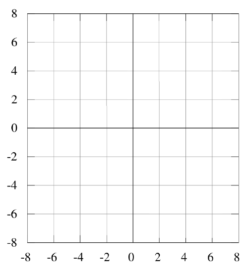
On the plot below, draw the potential energy for the harmonic oscillator (pick an arbitrary \(k\)) and draw the true ground-state wavefucntion for this potential and the trial wavefunction from Equation \ref{W8}. How does the trial wavefunction resemble the true wavefunction and not resemble the true wavefunction?

Q3
To obtain the energy, \(E_\phi\) for this trial wavefunction, we must calculate \(E_\phi\) from Equation \(\ref{W1}\). Break this into parts to make it more manageable. Start with the denominator. Write down the integral represented by \(\langle\phi|\phi\rangle\) using the trial wavefunction in Equation \(\ref{W8}\). what are the limits for this integral?
Q4
Use the mini-integral table above to solve the integral for \(\langle\phi |\phi\rangle\).
Q5
Is \(|\phi \rangle \) normalized? Does this matter (why or why not)?
Q6
The numerator for \(E_\phi\) in Equation \(\ref{W1}\) is \(\langle\phi|\hat H|\phi\rangle\). Write down the integral represented by \(\langle\phi|\hat H|\phi\rangle\) using the trial wavefunction in Equation \(\ref{W8}\), \(|\phi (x) \rangle\). What are the limits for the integral?
Q7
To solve the integral, the Hamiltonian must operate on the wavefunction. What is \(\hat H\) for this problem?
Q8
What do you get when you allow \(\hat H\) to operate on \(\phi\), what is, \(\hat H|\phi\rangle\)? Is \(\phi\) an eigenfunction of \(\hat H\)? Should it be an eigenfunction of \(\hat H\)?
Q9
Using your expression of \(\hat H|\phi \rangle \), write down the integral represented by at \(\langle\phi|\hat H|\phi\rangle\).
Q10
Now use the integrals above to solve for \(\langle\phi|\hat H|\phi\rangle\). It is good to break this into parts to solve.
Q11
Now put your whole answer together to get \(E_\phi=\dfrac{\langle\phi|\hat H|\phi\rangle}{\langle\phi|\phi\rangle}\). Your energy should be a function of \(\beta\).
The continuation of this Workgroup activity can be found in Variation Approximation II.

