
8.4: An Electron Has An Intrinsic Spin Angular Momentum
- Page ID
- 92403
\( \newcommand{\vecs}[1]{\overset { \scriptstyle \rightharpoonup} {\mathbf{#1}} } \)
\( \newcommand{\vecd}[1]{\overset{-\!-\!\rightharpoonup}{\vphantom{a}\smash {#1}}} \)
\( \newcommand{\id}{\mathrm{id}}\) \( \newcommand{\Span}{\mathrm{span}}\)
( \newcommand{\kernel}{\mathrm{null}\,}\) \( \newcommand{\range}{\mathrm{range}\,}\)
\( \newcommand{\RealPart}{\mathrm{Re}}\) \( \newcommand{\ImaginaryPart}{\mathrm{Im}}\)
\( \newcommand{\Argument}{\mathrm{Arg}}\) \( \newcommand{\norm}[1]{\| #1 \|}\)
\( \newcommand{\inner}[2]{\langle #1, #2 \rangle}\)
\( \newcommand{\Span}{\mathrm{span}}\)
\( \newcommand{\id}{\mathrm{id}}\)
\( \newcommand{\Span}{\mathrm{span}}\)
\( \newcommand{\kernel}{\mathrm{null}\,}\)
\( \newcommand{\range}{\mathrm{range}\,}\)
\( \newcommand{\RealPart}{\mathrm{Re}}\)
\( \newcommand{\ImaginaryPart}{\mathrm{Im}}\)
\( \newcommand{\Argument}{\mathrm{Arg}}\)
\( \newcommand{\norm}[1]{\| #1 \|}\)
\( \newcommand{\inner}[2]{\langle #1, #2 \rangle}\)
\( \newcommand{\Span}{\mathrm{span}}\) \( \newcommand{\AA}{\unicode[.8,0]{x212B}}\)
\( \newcommand{\vectorA}[1]{\vec{#1}} % arrow\)
\( \newcommand{\vectorAt}[1]{\vec{\text{#1}}} % arrow\)
\( \newcommand{\vectorB}[1]{\overset { \scriptstyle \rightharpoonup} {\mathbf{#1}} } \)
\( \newcommand{\vectorC}[1]{\textbf{#1}} \)
\( \newcommand{\vectorD}[1]{\overrightarrow{#1}} \)
\( \newcommand{\vectorDt}[1]{\overrightarrow{\text{#1}}} \)
\( \newcommand{\vectE}[1]{\overset{-\!-\!\rightharpoonup}{\vphantom{a}\smash{\mathbf {#1}}}} \)
\( \newcommand{\vecs}[1]{\overset { \scriptstyle \rightharpoonup} {\mathbf{#1}} } \)
\( \newcommand{\vecd}[1]{\overset{-\!-\!\rightharpoonup}{\vphantom{a}\smash {#1}}} \)
\(\newcommand{\avec}{\mathbf a}\) \(\newcommand{\bvec}{\mathbf b}\) \(\newcommand{\cvec}{\mathbf c}\) \(\newcommand{\dvec}{\mathbf d}\) \(\newcommand{\dtil}{\widetilde{\mathbf d}}\) \(\newcommand{\evec}{\mathbf e}\) \(\newcommand{\fvec}{\mathbf f}\) \(\newcommand{\nvec}{\mathbf n}\) \(\newcommand{\pvec}{\mathbf p}\) \(\newcommand{\qvec}{\mathbf q}\) \(\newcommand{\svec}{\mathbf s}\) \(\newcommand{\tvec}{\mathbf t}\) \(\newcommand{\uvec}{\mathbf u}\) \(\newcommand{\vvec}{\mathbf v}\) \(\newcommand{\wvec}{\mathbf w}\) \(\newcommand{\xvec}{\mathbf x}\) \(\newcommand{\yvec}{\mathbf y}\) \(\newcommand{\zvec}{\mathbf z}\) \(\newcommand{\rvec}{\mathbf r}\) \(\newcommand{\mvec}{\mathbf m}\) \(\newcommand{\zerovec}{\mathbf 0}\) \(\newcommand{\onevec}{\mathbf 1}\) \(\newcommand{\real}{\mathbb R}\) \(\newcommand{\twovec}[2]{\left[\begin{array}{r}#1 \\ #2 \end{array}\right]}\) \(\newcommand{\ctwovec}[2]{\left[\begin{array}{c}#1 \\ #2 \end{array}\right]}\) \(\newcommand{\threevec}[3]{\left[\begin{array}{r}#1 \\ #2 \\ #3 \end{array}\right]}\) \(\newcommand{\cthreevec}[3]{\left[\begin{array}{c}#1 \\ #2 \\ #3 \end{array}\right]}\) \(\newcommand{\fourvec}[4]{\left[\begin{array}{r}#1 \\ #2 \\ #3 \\ #4 \end{array}\right]}\) \(\newcommand{\cfourvec}[4]{\left[\begin{array}{c}#1 \\ #2 \\ #3 \\ #4 \end{array}\right]}\) \(\newcommand{\fivevec}[5]{\left[\begin{array}{r}#1 \\ #2 \\ #3 \\ #4 \\ #5 \\ \end{array}\right]}\) \(\newcommand{\cfivevec}[5]{\left[\begin{array}{c}#1 \\ #2 \\ #3 \\ #4 \\ #5 \\ \end{array}\right]}\) \(\newcommand{\mattwo}[4]{\left[\begin{array}{rr}#1 \amp #2 \\ #3 \amp #4 \\ \end{array}\right]}\) \(\newcommand{\laspan}[1]{\text{Span}\{#1\}}\) \(\newcommand{\bcal}{\cal B}\) \(\newcommand{\ccal}{\cal C}\) \(\newcommand{\scal}{\cal S}\) \(\newcommand{\wcal}{\cal W}\) \(\newcommand{\ecal}{\cal E}\) \(\newcommand{\coords}[2]{\left\{#1\right\}_{#2}}\) \(\newcommand{\gray}[1]{\color{gray}{#1}}\) \(\newcommand{\lgray}[1]{\color{lightgray}{#1}}\) \(\newcommand{\rank}{\operatorname{rank}}\) \(\newcommand{\row}{\text{Row}}\) \(\newcommand{\col}{\text{Col}}\) \(\renewcommand{\row}{\text{Row}}\) \(\newcommand{\nul}{\text{Nul}}\) \(\newcommand{\var}{\text{Var}}\) \(\newcommand{\corr}{\text{corr}}\) \(\newcommand{\len}[1]{\left|#1\right|}\) \(\newcommand{\bbar}{\overline{\bvec}}\) \(\newcommand{\bhat}{\widehat{\bvec}}\) \(\newcommand{\bperp}{\bvec^\perp}\) \(\newcommand{\xhat}{\widehat{\xvec}}\) \(\newcommand{\vhat}{\widehat{\vvec}}\) \(\newcommand{\uhat}{\widehat{\uvec}}\) \(\newcommand{\what}{\widehat{\wvec}}\) \(\newcommand{\Sighat}{\widehat{\Sigma}}\) \(\newcommand{\lt}{<}\) \(\newcommand{\gt}{>}\) \(\newcommand{\amp}{&}\) \(\definecolor{fillinmathshade}{gray}{0.9}\)- Understand the forth quantum number for electrons - spin.
- Understand how spin is connected to magnetic properties of the electrons and atoms.
- Understand how to break degeneracy via externally applied magnetic fields in electrons and atoms.
Imagine doing a hypothetical experiment that would lead to the discovery of electron spin. Your laboratory has just purchased a microwave spectrometer with variable magnetic field capacity. We try the new instrument with hydrogen atoms using a magnetic field of 104 Gauss and look for the absorption of microwave radiation as we scan the frequency of our microwave generator (Figure 8.4.1 ).

Finally we see absorption at a microwave photon frequency of \(28 \times 10^9\, Hz\) (28 gigahertz). This result is really surprising from several perspectives. Each hydrogen atom is in its ground state, with the electron in a 1s orbital. The lowest energy electronic transition that we predict based on existing theory (the electronic transition from the ground state (\(\psi _{100}\) to \(\psi _{21m}\)) requires an energy that lies in the vacuum ultraviolet (the lower Lyman line at 121 nm), not the microwave, region of the spectrum. Furthermore, when we vary the magnetic field we note that the frequency at which the absorption occurs varies in proportion to the magnetic field.
The Zeeman Effect: Breaking Degeneracies with Magnetic Fields
Magnetism results from the circular motion of charged particles. This property is demonstrated on a macroscopic scale by making an electromagnet from a coil of wire and a battery. Electrons moving through the coil produce a magnetic field, which can be thought of as originating from a magnetic dipole or a bar magnet. Electrons in atoms also are moving charges with angular momentum so they too produce a magnetic dipole, which is why some materials are magnetic. A magnetic dipole interacts with a magnetic field, and the energy of this interaction is given by the scalar product of the magnetic dipole moment, and the magnetic field, \(\vec{B}\).
\[E_B = -\vec{\mu}_m \cdot \vec{B} \label {8.4.0} \]
Pieter Zeeman was one of the first to observe the splittings of spectral lines in a magnetic field caused by this interaction. Consequently such splittings are known as the Zeeman effect. (Figure 8.4.2 ). The expectation value calculated for the total energy in this case is the sum of the energy in the absence of the field, \(E_n\), plus the Zeeman energy:
\[\begin{align} \left \langle E \right \rangle &= E_n + \dfrac {e \hbar B_z m_l}{2m_e} \\[4pt] &= E_n + \mu _B B_z m_l \label {8.4.13} \end{align} \]
The factor
\[ \dfrac {e \hbar}{2m_e} = - \gamma _e \hbar = \mu _B \label {8.4.14} \]
defines the constant \(\mu _B\), called the Bohr magneton, which is taken to be the fundamental magnetic moment. It has units of \(9.2732 \times 10^{-21}\) erg/Gauss or \(9.2732 \times 10^{-24}\) Joule/Tesla. This factor will help you to relate magnetic fields, measured in Gauss or Tesla, to energies, measured in ergs or Joules, for any particle with a charge and mass the same as an electron.
Equation \ref{8.4.13} demonstrates that that \(m_l\) quantum number degeneracy of the hydrogen atom is removed by the externally applied magnetic field. For example, the three hydrogen atom eigenstates \(|\psi _{211} \rangle\), \(|\psi _{21-1} \rangle\), and \(|\psi _{210} \rangle \) are degenerate in zero magnetic field, but have different energies in an externally applied magnetic field (Figure 8.4.2 ).

The \(m_l = 0\) state, for which the component of angular momentum and hence also the magnetic moment in the external field direction is zero, experiences no interaction with the magnetic field. The \(m_l = +1\) state, for which the angular momentum in the z-direction is +ħ and the magnetic moment is in the opposite direction, against the field, experiences a raising of energy in the presence of a field. Maintaining the magnetic dipole against the external field direction is like holding a small bar magnet with its poles aligned exactly opposite to the poles of a large magnet. It is a higher energy situation than when the magnetic moments are aligned with each other.
Electron Spin and the Stern-Gerlach Experiment
To discover new things, experimentalists sometimes must explore new areas in spite of contrary theoretical predictions. Our theory of the hydrogen atom at this point gives no reason to look for absorption in the microwave region of the spectrum. By doing the crazy experiment outlines above, we discovered that when an electron is in the \(|1s \rangle\) orbital of the hydrogen atom, there are two different states that have the same energy. When a magnetic field is applied, this degeneracy is removed, and microwave radiation can cause transitions between the two states. In the rest of this section, we see what can be deduced from this experimental observation. This experiment actually could be done with electron spin resonance spectrometers available today (Figure 8.4.1 ). To explain our observations, a new model for the hydrogen atom. Our original model for the hydrogen atom accounted for the motion of the electron and proton in our three-dimensional world; the new model needs something else that can give rise to an additional Zeeman-like effect. We need a charged particle with angular momentum to produce a magnetic moment, just like that obtained by the orbital motion of the electron. We can postulate that our observation results from a motion of the electron that was not considered in the last section - electron spin. We have a charged particle spinning on its axis. We then have charge moving in a circle, angular momentum, and a magnetic moment, which interacts with the magnetic field and gives us the Zeeman-like effect that we observed (Figure 8.4.2 ).

In 1920, Otto Stern and Walter Gerlach designed an experiment, which unintentionally led to the discovery that electrons have their own individual, continuous spin even as they move along their orbital of an atom. Today, this electron spin is indicated by the fourth quantum number, also known as the Electron Spin Quantum Number and denoted by \(m_s\). In 1925, Samuel Goudsmit and George Uhlenbeck made the claim that features of the hydrogen spectrum that were unexamined might by explained by assuming electrons act as if it has a spin, which can be denoted by an arrow pointing up, which is +1/2, or an arrow pointing down, which is -1/2. The Stern and Gerlach experiment which demonstrated this was done with a beam of vaporized silver atoms that split into two beams after passing through a magnetic field (Figure 8.4.2 ). An explanation of this is that an electron has a magnetic field due to its spin. When electrons that have opposite spins are put together, there is no net magnetic field because the positive and negative spins cancel each other out. The silver atom used in the experiment has a total of 47 electrons, 23 of one spin type, and 24 of the opposite. Because electrons of the same spin cancel each other out, the one unpaired electron in the atom will determine the spin.
Spin Eigenstates and Eigenvalues
To describe electron spin from a quantum mechanical perspective, we must have spin wavefunctions and spin operators. The properties of the spin states are deduced from experimental observations and by analogy with our treatment of the states arising from the orbital angular momentum of the electron. The important feature of the spinning electron is the spin angular momentum vector, which we label \(S\) by analogy with the orbital angular momentum \(L\). We define spin angular momentum operators with the same properties that we found for the rotational and orbital angular momentum operators. After all, angular momentum is angular momentum, no matter if it is orbital or spin in nature.
We found that
\[ \hat {L}^2 | Y^{m_l} _l \rangle = l(l + 1) \hbar^2 | Y^{m_l}_l \rangle \nonumber \]
so by analogy for the spin states, we must have
\[ \hat {S}^2 | \sigma ^{m_s} _s \rangle = s( s + 1) \hbar ^2 | \sigma ^{m_s}_s \rangle \nonumber \]
where \(\sigma\) is a spin wavefunction with quantum numbers \(s\) and \(m_s\) that obey the same rules as the quantum numbers \(l\) and \(m_l\) associated with the spherical harmonic wavefunction \(Y\). We also found the project of the orbital angular momentum on the z-axis is
\[ \hat {L}_z | Y^{m_l}_l \rangle = m_l \hbar | Y^{m_l}_l \rangle \nonumber \]
so by analogy, we must have a similar projection for the spin angular momentum:
\[ \hat {S}_z | \sigma ^{m_s}_s \rangle = m_s \hbar | \sigma ^{m_s}_s \rangle \label {8.4.4} \]
Since \(m_l\) ranges in integer steps from \(-l\) to \(+l\), also by analogy \(m_s\) ranges in integer steps from \(-s\) to \(+s\). In our hypothetical experiment, we observed one absorption transition, which means there are two spin states. Consequently, the two values of \(m_s\) must be \(+s\) and \(-s\), and the difference in \(m_s\) for the two states, labeled f and i below, must be the smallest integer step, i.e., 1. The result of this logic is that
\[\begin{align} m_{s,f} - m_{s,i} &= 1 \nonumber\\[4pt] (+s) - (-s) &= 1 \nonumber\\[4pt] 2s &= 1 \nonumber\\[4pt] s &= \dfrac {1}{2} \label {8.4.5} \end{align} \]
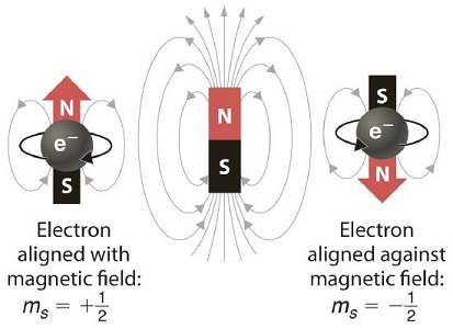
Therefore our conclusion is that the magnitude of the spin quantum number is 1/2 and the values for \(m_s\) are +1/2 and -1/2. The two spin states correspond to spinning clockwise and counter-clockwise with positive and negative projections of the spin angular momentum onto the z-axis (Figure 8.4.3 ). The state with a positive projection, \(m_s\) = +1/2, is called \(\alpha\); the other is called \(\beta\). These spin states are arbitrarily labeled \(\alpha\) and \(\beta\), and the associated spin wavefunctions also are designated by \(|\alpha \rangle \) and \(| \beta \rangle\).
From Equation \(\ref{8.4.4}\), the magnitude of the z-component of spin angular momentum, \(S_z\), is given by
\[S_z = m_s \hbar \label {8.4.6} \]
so the value of \(S_z\) is \(+ħ/2\) for spin state \(\alpha\) and \(-ħ/2\) for spin state \(\beta\). Hence, we conclude that the \(\alpha\) spin state, where the magnetic moment is aligned against the external field direction, has a greater energy than the \(\beta\) spin state.
Electron's hypothetical surface would have to be moving faster than the speed of light for it to rotate quickly enough to produce the observed angular momentum. Hence, an electron is not simply a spinning ball or ring and electron spin appears to be an intrinsic angular moment of the particle rather than a consequence of the rotation of a charge particle like Figure 8.4.3 suggests. Despite this, the term "electron spin" persists in quantum vernacular.
Even though we do not know their functional forms, the spin wavefunctions are taken to be normalized and orthogonal to each other.
\[ \int \alpha ^* \alpha \,d \tau _s = \int \beta ^* \beta \,d \tau _s = 1 \label {8.4.7a} \]
or in braket notation
\[ \langle \alpha | \alpha \rangle = \langle \beta | \beta \rangle =1 \label{8.4.7b} \]
and
\[ \int \alpha ^* \beta\, d \tau _s = \int \beta ^* \alpha\, d \tau _s = 0 \label {8.4.8a} \]
or in braket notation
\[ \langle \alpha | \beta \rangle = \langle \alpha | \beta \rangle = 0 \label{8.4.8b} \]
where the integral is over the spin variable \(\tau _s\).
Now let's apply these deductions to the experimental observations in our hypothetical microwave experiment in Figure 8.4.1 . We can account for the frequency of the transition (\(\nu\)= 28 gigahertz) that was observed in this hypothetical experiment in terms of the magnetic moment of the spinning electron and the strength of the magnetic field. The photon energy, \(h \nu\), is given by the difference between the energies of the two states, \(E_{\alpha}\) and \(E_{\beta}\)
\[\begin{align} \Delta E &= h \nu \\[4pt] &= E_{\alpha} - E_{\beta} \label {8-49}\end{align} \]
The energies of these two states consist of the sum of the energy of an electron in a 1s orbital, \(E_{1s}\), and the energy due to the interaction of the spin magnetic dipole moment of the electron, \(\mu _s\), with the magnetic field, \(B\).

The two states with distinct values for spin magnetic moment \(\mu _s\) are denoted by the subscripts \(\alpha\) and \(\beta\) (the spin version of Equation \ref{8.4.0}.
\[ \begin{align*} E_{\alpha} &= E_{1s} - \mu _{s,\alpha} \cdot B \\[4pt] E_{\beta} &= E_{1s} - \mu _{s,\beta} \cdot B \end{align*} \]
Substituting the two equations above into the expression for the photon (Equation \ref{8-49}) energy gives
\[\begin{align} h \nu &= E_{\alpha} - E_{\beta} \\[4pt] &= (E_{1s} - \mu _{s, \alpha} \cdot B) - (E_{1s} - \mu_{s,\beta} \cdot B) \label {8-52} \\[4pt] &= ( \mu _{s, \beta} - \mu _{s, \alpha}) \cdot B \label{8-53} \end{align} \]
Again by analogy with the orbital angular momentum and magnetic moment discussed above, we take the spin magnetic dipole of each spin state, \(\mu _{s, \alpha}\) and \(\mu _{s, \beta}\), to be related to the total spin angular momentum of each state, \(S_{\alpha}\) and \(S_{\beta}\), by a constant spin gyromagnetic ratio, \(\gamma _s\), as shown below.
\[ \mu _s = \gamma _s S \nonumber \]
or each of the two states
\[\mu _{s, \alpha} = \gamma _s S_\alpha \nonumber \]
\[\mu _{s, \beta} = \gamma _s S_\beta \nonumber \]
With the magnetic field direction defined as \(z\), the scalar product in Equation \ref{8-53} becomes a product of the z-components of the spin angular momenta, \(S_{z, \alpha}\) and \(S_{z, \beta}\), with the external magnetic field.
Inserting the values for \(S_{z,\alpha} = +\dfrac {1}{2} \hbar \) and \( S_{z, \alpha} = -\dfrac {1}{2} \hbar\) from Equation \ref{8.4.6} and rearranging Equation \ref{8-53} yields
\[ \dfrac {h \nu}{B} = - \gamma _s \hbar \nonumber \]
Calculating the ratio \(\dfrac {h \nu}{B}\) from our experimental results, \(\nu = 28 \times 10^9\, Hz\) when \(B = 10^4\, gauss\), gives us a value for
\[- \gamma_s \hbar = 18.5464 \times 10^{-21}\, erg/gauss. \nonumber \]
This value is about twice the Bohr magneton,\(-\gamma _e \hbar \), found in Equation \ref{8.4.14} i.e. \(\gamma _s \hbar = 2.0023, \gamma _e \hbar\), or
\[\gamma _s = 2.0023 \gamma _e \label \nonumber \]
The factor of 2.0023 is called the g-factor and accounts for the deviation of the spin gyromagnetic ratio from the value expected for orbital motion of the electron. In other words, it accounts for the spin transition being observed where it is instead of where it would be if the same ratio between magnetic moment and angular momentum held for both orbital and spin motions. The value 2.0023 applies to a freely spinning electron; the coupling of the spin and orbital motion of electrons can produce other values for \(g\).
Carry out the calculations that show that the g-factor for electron spin is 2.0023.
Interestingly, the concept of electron spin and the value g = 2.0023 follow logically from Dirac's relativistic quantum theory, which is beyond the scope of this discussion. Electron spin was introduced here as a postulate to explain experimental observations. Scientists often introduce such postulates parallel to developing the theory from which the property is naturally deduced.