Precode Loading
On the next cell we are going to import the libraries used in this notebook as well as call some important functions.
In the next cell we are shutting down eventual warnings displayed. This cell is optional.
Executing the next cell prints on the screen the versions of IPython, Python and its libraries on your computer. Please check if the versions are up-to-date to facilitate a smooth running of the program.
The next cell configures matplotlib to show figures embedded within the cells it was executed from, instead of opening a new window for each figure.
Particle in a 1D Box
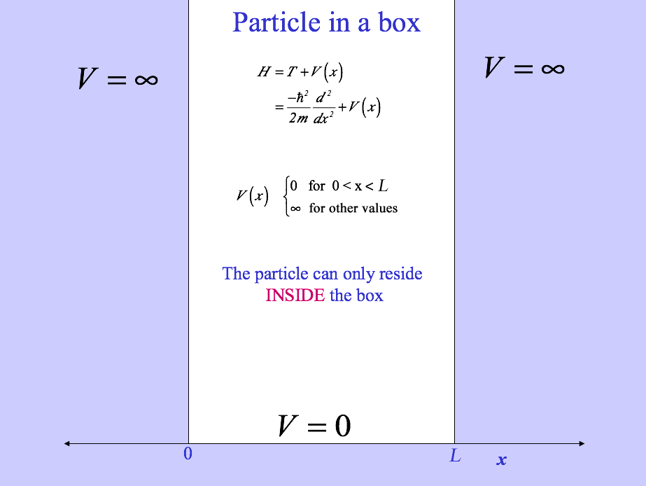
Inside the box, the potential is equal to zero, therefore the Schrödinger equation for this system is given by:
\[\frac{-\hbar^2}{2m}\frac{\partial^2\psi_n(x)}{\partial{x}^2} =E\psi_n(x) \]
Since the potential is infinity outside the box, the wavefunction must obey the following Boundary Condition:
\[\psi_n(0)=\psi_n(L)=0\]
where \(L\) is the length of the box.
After solving the Schrödinger equation, the normalized eigenfunctions obtained are given by:
\[\psi_n(x) = \sqrt{\frac{2}{L}} \sin\left(\frac{n\pi}{L}x\right) \label{eigenstates}\]
where \(n=1, 2, ..., \infty \).
It is important to emphasize that the quantization (\(n\) being only positive integers) is a consequence of the boundary conditions. Here are a few questions to think about before we move on:
Questions
- Q1: Can you infer, just looking at the graphical representations of \(\psi_n(x)\) or \(|\psi_n(x)|^2\), what is the quantum state (labeled by its quantum number) \(n\)?
- Q2: What is a node? How do the nodes relate to the Kinetic Energy of the system?
- Q3: Is it possible to find the particle outside the box?
- Q4: Does it matter that \(\psi_n(x)\) has negative values?
- Q5: What variables and parameters does \(\psi_n(x)\) depend on?
Some of these questions can be answered by plotting the Wavefunction, \(\psi_n(x)\) and the Probability Density, \(|\psi_n(x)|^2\) for different values of \(n\).
Wavefunctions and Probability Densities
import matplotlib.pyplot as plt
import numpy as np

# Defining the wavefunction
def psi(x,n,L): return np.sqrt(2.0/L)*np.sin(float(n)*np.pi*x/L)

# Reading the input variables from the user
n = int(input("Enter the value for the quantum number n = "))
L = float(input("Enter the size of the box in Angstroms = "))

# Generating the wavefunction graph
plt.rcParams.update({'font.size': 18, 'font.family': 'STIXGeneral', 'mathtext.fontset': 'stix'})
x = np.linspace(0, L, 900)
fig, ax = plt.subplots()
lim1=np.sqrt(2.0/L) # Maximum value of the wavefunction
ax.axis([0.0,L,-1.1*lim1,1.1*lim1]) # Defining the limits to be plot in the graph
str1=r"$n = "+str(n)+r"$"
ax.plot(x, psi(x,n,L), linestyle='--', label=str1, color="orange", linewidth=2.8) # Plotting the wavefunction
ax.hlines(0.0, 0.0, L, linewidth=1.8, linestyle='--', color="black") # Adding a horizontal line at 0
# Now we define labels, legend, etc
ax.legend(loc=2);
ax.set_xlabel(r'$L$')
ax.set_ylabel(r'$\psi_n(x)$')
plt.title('Wavefunction')
plt.legend(bbox_to_anchor=(1.1, 1), loc=2, borderaxespad=0.0)

# Generating the probability density graph
fig, ax = plt.subplots()
ax.axis([0.0,L,0.0,lim1*lim1*1.1])
str1=r"$n = "+str(n)+r"$"
ax.plot(x, psi(x,n,L)*psi(x,n,L), label=str1, linewidth=2.8)
ax.legend(loc=2);
ax.set_xlabel(r'$L$')
ax.set_ylabel(r'$|\psi_n|^2(x)$')
plt.title('Probability Density')
plt.legend(bbox_to_anchor=(1.1, 1), loc=2, borderaxespad=0.0)

# Show the plots on the screen once the code reaches this point
plt.show()
Length Dependence on Wavefunctions
We can explore the changes in the Wavefunction and Probability Density for a given state n in boxes of different length \(L\):
Wavefunctions and Probability Densities as a Function of size of Box
import matplotlib.pyplot as plt
import numpy as np

# Reading the input boxes sizes from the user, and making sure the values are not larger than 20 A
L = 100.0
while(L>20.0):
    L1 = float(input(" To compare wavefunctions for boxes of different lengths \nenter the value of L for the first box  (in Angstroms and not larger then 20 A) = "))
    L2 = float(input("Enter the value of L for the second box (in Angstroms and not larger then 20) = "))
    L = max(L1,L2)
    if(L>20.0):
        print ("The sizes of the boxes cannot be larger than 20 A. Please enter the values again.\n")

# Generating the wavefunction and probability density graphs
plt.rcParams.update({'font.size': 18, 'font.family': 'STIXGeneral', 'mathtext.fontset': 'stix'})
fig, ax = plt.subplots(figsize=(12,6))
ax.spines['right'].set_color('none')
ax.xaxis.tick_bottom()
ax.spines['left'].set_color('none')
ax.axes.get_yaxis().set_visible(False)
ax.spines['top'].set_color('none')
val = 1.1*max(L1,L2)
X1 = np.linspace(0.0, L1, 900,endpoint=True)
X2 = np.linspace(0.0, L2, 900,endpoint=True)
ax.axis([-0.5*val,1.5*val,-np.sqrt(2.0/L),3*np.sqrt(2.0/L)])
ax.set_xlabel(r'$X$ (Angstroms)')
strA="$\psi_n$"
strB="$|\psi_n|^2$"
ax.text(-0.12*val, 0.0, strA, rotation='vertical', fontsize=30, color="black")
ax.text(-0.12*val, np.sqrt(4.0/L), strB, rotation='vertical', fontsize=30, color="black")
str1=r"$L = "+str(L1)+r"$ A"
str2=r"$L = "+str(L2)+r"$ A"
ax.plot(X1,psi(X1,n,L1)*np.sqrt(L1/L), color="red", label=str1, linewidth=2.8)
ax.plot(X2,psi(X2,n,L2)*np.sqrt(L2/L), color="blue", label=str2, linewidth=2.8)
ax.plot(X1,psi(X1,n,L1)*psi(X1,n,L1)*(L1/L) + np.sqrt(4.0/L), color="red", linewidth=2.8)
ax.plot(X2,psi(X2,n,L2)*psi(X2,n,L2)*(L2/L) + np.sqrt(4.0/L), color="blue", linewidth=2.8)
ax.margins(0.00)
ax.legend(loc=9)
str2="$V = +\infty$"
ax.text(-0.3*val, 0.5*np.sqrt(2.0/L), str2, rotation='vertical', fontsize=40, color="black")
ax.vlines(0.0, -np.sqrt(2.0/L), 2.5*np.sqrt(2.0/L), linewidth=4.8, color="red")
ax.vlines(L1, -np.sqrt(2.0/L), 2.5*np.sqrt(2.0/L), linewidth=4.8, color="red")
ax.vlines(0.0, -np.sqrt(2.0/L), 2.5*np.sqrt(2.0/L), linewidth=4.8, color="blue")
ax.vlines(L2, -np.sqrt(2.0/L), 2.5*np.sqrt(2.0/L), linewidth=4.8, color="blue")
ax.hlines(0.0, 0.0, L, linewidth=1.8, linestyle='--', color="black")
ax.hlines(np.sqrt(4.0/L), 0.0, L, linewidth=1.8, linestyle='--', color="black")
plt.title('Wavefunction and Probability Density', fontsize=30)
str3=r"$n = "+str(n)+r"$"
ax.text(1.1*L,np.sqrt(4.0/L), r"$n = "+str(n)+r"$", fontsize=25, color="black")
plt.legend(bbox_to_anchor=(0.73, 0.95), loc=2, borderaxespad=0.)

# Show the plots on the screen once the code reaches this point
plt.show()
Energies
We can also look at the allowed values of energy, given by:
\[E_n = \frac{n^2 h^2}{8mL^2} \label{energy}\]
where \(m\) is the mass of the particle.
Note: Did you notice that \(\psi_n(x)\) does not depend on the mass of the particle (Equation \ref{eigenstates}), but the energies do (Equation \ref{energy})?
In contrast to the solution in the free particle system, for a particle confined within the box, not every energy value is allowed. We see that quantization is a direct consequence of the boundary condition. In other words: confinement leads to quantization.
Let's now analyze how the Energy Levels \(E_n\) for an electron change as a function of the size of the box.
Energy Levels as a Function of the Size of the Box
import matplotlib.pyplot as plt
#Given the following parameters

h=6.62607e-34    #planck's constant in joules
me=9.1093837e-31  # mass of an electron in kg
# (h**2 / (me*8))* (1e10)**2 *6.242e+18  #is the prefactor using length units is Angstroms and then converted into electron volts

# Defining a function to compute the energy

def En(n,L,m): return (h**2 / (m*8))* (1e10)**2 *6.242e+18*((float(n)/L)**2)

# Reading the input variables from the user
L1 = float(input(" To see how the energy levels change for boxes of different lengths, \nenter the value for L for the first box (in Angstroms) = "))
nmax1 = int(input("Enter the number of levels you want to plot for the first box = "))
L2 = float(input("Enter the value for L for the second box (in Angstroms) = "))
nmax2 = int(input("Enter the number of levels you want to plot for the second box = "))

# Generating the graph
plt.rcParams.update({'font.size': 18, 'font.family': 'STIXGeneral', 'mathtext.fontset': 'stix'})
fig, ax = plt.subplots(figsize=(8,12))
ax.spines['right'].set_color('none')
ax.yaxis.tick_left()
ax.spines['bottom'].set_color('none')
ax.axes.get_xaxis().set_visible(False)
ax.spines['top'].set_color('none')
val = 1.1*max(En(nmax1,L1,me),En(nmax2,L2,me))
val2= 1.1*max(L1,L2)
ax.axis([0.0,10.0,0.0,val])
ax.set_ylabel(r'$E_n$ (eV)')
for n in range(1,nmax1+1):
    str1="$n = "+str(n)+r"$, $E_{"+str(n)+r"} = %.3f$ eV"%(En(n,L1,me))
    ax.text(0.6, En(n,L1,me)+0.01*val, str1, fontsize=16, color="red")
    ax.hlines(En(n,L1,me), 0.0, 4.5, linewidth=1.8, linestyle='--', color="red")
for n in range(1,nmax2+1):
    str1="$n = "+str(n)+r"$, $E_{"+str(n)+r"} = %.3f$ eV"%(En(n,L2,me))
    ax.text(6.2, En(n,L2,me)+0.01*val, str1, fontsize=16, color="blue")
    ax.hlines(En(n,L2,me), 5.5, 10.0, linewidth=1.8, linestyle='--', color="blue")
str1=r"$L = "+str(L1)+r"$ A"
plt.title("Energy Levels for a particle of mass = $m_{electron}$ \n ", fontsize=30)
str1=r"$L = "+str(L1)+r"$ A"
str2=r"$L = "+str(L2)+r"$ A"
ax.text(1.5,val, str1, fontsize=25, color="red")
ax.text(6,val, str2, fontsize=25, color="blue")

# Show the plots on the screen once the code reaches this point
plt.show()
and how the Energy Levels, \(E_n\) change as a function of the mass of the particle.
Energy Levels as a Function of the Mass of Particle
import matplotlib.pyplot as plt

# Reading the input variables from the user
L = float(input(" Enter the value for L for both boxes (in Angstroms) = "))
m1 = float(input(" To see how the energy levels change for particles of different mass, \nEnter the value of the mass for the first particle (in units of the mass of 1 electron) = "))
nmax1 = int(input("Enter the number of levels you want to plot for the first box = "))
m2 = float(input("Enter the value of the mass for the second particle (in units of the mass of 1 electron) = "))
nmax2 = int(input("Enter the number of levels you want to plot for the second box = "))

# Generating the graph
plt.rcParams.update({'font.size': 18, 'font.family': 'STIXGeneral', 'mathtext.fontset': 'stix'})
fig, ax = plt.subplots(figsize=(8,12))
ax.spines['right'].set_color('none')
ax.yaxis.tick_left()
ax.spines['bottom'].set_color('none')
ax.axes.get_xaxis().set_visible(False)
ax.spines['top'].set_color('none')
val = 1.1*max(En(nmax1,L,m1*me),En(nmax2,L,m2*me))
val2= 1.1*max(m1,m2)
ax.axis([0.0,10.0,0.0,val])
ax.set_ylabel(r'$E_n$ (eV)')
for n in range(1,nmax1+1):
    str1="$n = "+str(n)+r"$, $E_{"+str(n)+r"} = %.3f$ eV"%(En(n,L,m1*me))
    ax.text(0.6, En(n,L,m1*me)+0.01*val, str1, fontsize=16, color="green")
    ax.hlines(En(n,L,m1*me), 0.0, 4.5, linewidth=1.8, linestyle='--', color="green")
for n in range(1,nmax2+1):
    str1="$n = "+str(n)+r"$, $E_{"+str(n)+r"} = %.3f$ eV"%(En(n,L,m2*me))
    ax.text(6.2, En(n,L,m2*me)+0.01*val, str1, fontsize=16, color="magenta")
    ax.hlines(En(n,L,m2*me), 5.5, 10.0, linewidth=1.8, linestyle='--', color="magenta")
str1=r"$m = "+str(m1)+r"$ A"
plt.title("Energy Levels for two particles with different masses\n ", fontsize=30)
str1=r"$m_1 = "+str(m1)+r"$ $m_e$ "
str2=r"$m_2 = "+str(m2)+r"$ $m_e$ "
ax.text(1.1,val, str1, fontsize=25, color="green")
ax.text(6.5,val, str2, fontsize=25, color="magenta")

# Show the plots on the screen once the code reaches this point
plt.show()
We can combine the information from the wavefunctions, probability density, and energies into a single plot that compares the wavefunctions and the probability densities for different states, each one represented at its energy value. These plots are made using the electron mass.
Combined presentation of Energy Levels, Wavefunctions and Probability Densities
import matplotlib.pyplot as plt
import numpy as np

# Here the users inputs the value of L
L = float(input("Enter the value of L (in Angstroms) = "))
nmax = int(input("Enter the maximum value of n you want to plot = "))

# Generating the wavefunction graph
fig, ax = plt.subplots(figsize=(12,9))
ax.spines['right'].set_color('none')
ax.xaxis.tick_bottom()
ax.spines['left'].set_color('none')
ax.axes.get_yaxis().set_visible(False)
ax.spines['top'].set_color('none')
X3 = np.linspace(0.0, L, 900,endpoint=True)
Emax = En(nmax,L,me)
amp = (En(2,L,me)-En(1,L,me)) *0.9
Etop = (Emax+amp)*1.1
ax.axis([-0.5*L,1.5*L,0.0,Etop])
ax.set_xlabel(r'$X$ (Angstroms)')

for n in range(1,nmax+1):
    ax.hlines(En(n,L,me), 0.0, L, linewidth=1.8, linestyle='--', color="black")
    str1="$n = "+str(n)+r"$, $E_{"+str(n)+r"} = %.3f$ eV"%(En(n,L,me))
    ax.text(1.03*L, En(n,L,me), str1, fontsize=16, color="black")
    ax.plot(X3,En(n,L,me)+amp*np.sqrt(L/2.0)*psi(X3,n,L), color="red", label="", linewidth=2.8)
ax.margins(0.00)
ax.vlines(0.0, 0.0, Etop, linewidth=4.8, color="blue")
ax.vlines(L, 0.0, Etop, linewidth=4.8, color="blue")
ax.hlines(0.0, 0.0, L, linewidth=4.8, color="blue")
plt.title('Wavefunctions', fontsize=30)
plt.legend(bbox_to_anchor=(0.8, 1), loc=2, borderaxespad=0.)
str2="$V = +\infty$"
ax.text(-0.15*L, 0.6*Emax, str2, rotation='vertical', fontsize=40, color="black")

# Generating the probability density graph
fig, ax = plt.subplots(figsize=(12,9))
ax.spines['right'].set_color('none')
ax.xaxis.tick_bottom()
ax.spines['left'].set_color('none')
ax.axes.get_yaxis().set_visible(False)
ax.spines['top'].set_color('none')
X3 = np.linspace(0.0, L, 900,endpoint=True)
Emax = En(nmax,L,me)
ax.axis([-0.5*L,1.5*L,0.0,Etop])
ax.set_xlabel(r'$X$ (Angstroms)')
for n in range(1,nmax+1):
    ax.hlines(En(n,L,me), 0.0, L, linewidth=1.8, linestyle='--', color="black")
    str1="$n = "+str(n)+r"$, $E_{"+str(n)+r"} = %.3f$ eV"%(En(n,L,me))
    ax.text(1.03*L, En(n,L,me), str1, fontsize=16, color="black")
    ax.plot(X3,En(n,L,me)+ amp*(np.sqrt(L/2.0)*psi(X3,n,L))**2, color="red", label="", linewidth=2.8)
ax.margins(0.00)
ax.vlines(0.0, 0.0, Etop, linewidth=4.8, color="blue")
ax.vlines(L, 0.0, Etop, linewidth=4.8, color="blue")
ax.hlines(0.0, 0.0, L, linewidth=4.8, color="blue")
plt.title('Probability Density', fontsize=30)
plt.legend(bbox_to_anchor=(0.8, 1), loc=2, borderaxespad=0.)
str2="$V = +\infty$"
ax.text(-0.15*L, 0.6*Emax, str2, rotation='vertical', fontsize=40, color="black")

# Show the plots on the screen once the code reaches this point
plt.show()
Once we know the properties of a 1D box, we can use separation of variables to find the solutions to the 2D and 3D box problem.
Particle in a 2D box
Since the 2-D Hamiltonian can be separated into two 1-D Hamiltonians, one depending only on the variable x and one depending only on the variable y, the solution to the 2D Schrödinger equation will be a wavefunction that is the product of the 1D solutions in the x and y directions with independent quantum numbers \(n\) and \(m\):
\[\begin{align*} \Psi_{n,m}(x,y) &= \psi_{n}(x) \ \psi_{m}(y) \\[4pt] &=\frac{2}{\sqrt{L_xL_y}} \sin\left(\frac{n\pi}{L_x}x\right) \; \sin\left(\frac{m\pi}{L_y}y\right) \end{align*}\]
Wavefunctions for a Particle in a 2D Box as a Function of the Quantum numbers
Since the variables are independent, a vertical slice in this plot shows the y dependence of the wavefunction, thus it would look like a 1D particle in a box. Similarly, a horizontal slice gives the x dependence, and behaves as a 1D wavefunction. Let's see that:
Slices Through Wavefunctions for a Particle in a 2D Box
import matplotlib.pyplot as plt
import numpy as np

# Here the users inputs the values of n and m
yo = float(input("Enter the value of y/L_y for the x-axes slice ="))
xo = float(input("Enter the value of x/L_x for the y-axes slice ="))

# Generating the wavefunction graph
plt.rcParams.update({'font.size': 18, 'font.family': 'STIXGeneral', 'mathtext.fontset': 'stix'})
x = np.linspace(0, 1.0, 900)
fig, ax = plt.subplots()
lim1=2.0 # Maximum value of the wavefunction
ax.axis([0.0,1.0,-1.1*lim1,1.1*lim1]) # Defining the limits to be plot in the graph
str1=r"$n = "+str(n)+r", m = "+str(m)+r", y_o = "+str(yo)+r"\times L_y$"
ax.plot(x, psi2D(x,yo), linestyle='--', label=str1, color="orange", linewidth=2.8) # Plotting the wavefunction
ax.hlines(0.0, 0.0, 1.0, linewidth=1.8, linestyle='--', color="black") # Adding a horizontal line at 0
# Now we define labels, legend, etc
ax.legend(loc=2);
ax.set_xlabel(r'$x/L_x$')
ax.set_ylabel(r'$\sqrt{L_xL_y}\Psi_{n,m}(x,y_o)$')
plt.legend(bbox_to_anchor=(1.1, 1), loc=2, borderaxespad=0.0)

# Generating the wavefunction graph
plt.rcParams.update({'font.size': 18, 'font.family': 'STIXGeneral', 'mathtext.fontset': 'stix'})
y = np.linspace(0, 1.0, 900)
fig, ax = plt.subplots()
lim1=2.0 # Maximum value of the wavefunction
ax.axis([0.0,1.0,-1.1*lim1,1.1*lim1]) # Defining the limits to be plot in the graph
str1=r"$n = "+str(n)+r", m = "+str(m)+r", x_o = "+str(xo)+r"\times L_x$"
ax.plot(y, psi2D(xo,y), linestyle='--', label=str1, color="blue", linewidth=2.8) # Plotting the wavefunction
ax.hlines(0.0, 0.0, 1.0, linewidth=1.8, linestyle='--', color="black") # Adding a horizontal line at 0
# Now we define labels, legend, etc
ax.legend(loc=2);
ax.set_xlabel(r'$y/L_y$')
ax.set_ylabel(r'$\sqrt{L_xL_y}\Psi_{n,m}(x_o,y)$')
plt.legend(bbox_to_anchor=(1.1, 1), loc=2, borderaxespad=0.0)

# Show the plots on the screen once the code reaches this point
plt.show()
Questions
Here are some questions to consider from the plots (answer for arbitrary values of quantum numbers):
- Q1: How many nodes does \(\Psi_{n,m}\) have in the x axis?
- Q2: How many nodes does \(\Psi_{n,m}\) have in the y axis?
- Q3: Can you sketch the equivalent plot for a non-symmetric box (for example, with \(L_x = 2L_y\))?
How about the energies?
When the Hamiltonian can be separated into independent Hamiltonians, the wavefunction can be built as the product of independent wavefunctions and the energy will be given by the sum of the 1D energies:
\[\begin{align*} E_{n,m} &= E_n +E_m \\[4pt] &= \frac{ h^2}{8m_p} \frac{n^2}{L_x^2}+ \frac{ h^2}{8m_p}\frac{m^2}{L_y^2} \\[4pt] &= \frac{ h^2}{8m_p}\left(\frac{n^2}{L_x^2}+\frac{m^2}{L_y^2}\right) \end{align*}\]
Depending on the values of \(L_x\) and \(L_y\) (the length of the box on each side), we may get degenerated states: more than one state with the same energy.
Let's look at these Energy Levels as a function of quantum numbers and box sizes:
Energy Levels as a Function of Quantum Numbers and Box Sizes
import matplotlib.pyplot as plt

# Defining the energy as a function
def En2D(n,m,L1,L2): return 37.60597*((float(n)/L1)**2+ (float(m)/L2)**2)

# Reading data from the user
L1 = float(input("Can we count DEGENERATE states?\nEnter the value for Lx (in Angstroms) = "))
nmax1 = int(input("Enter the maximum value of n to consider = "))
L2 = float(input("Enter the value for Ly (in Angstroms) = "))
mmax2 = int(input("Enter the maximum value of m to consider = "))

# Plotting the energy levels
plt.rcParams.update({'font.size': 18, 'font.family': 'STIXGeneral', 'mathtext.fontset': 'stix'})
fig, ax = plt.subplots(figsize=(nmax1*2+2,nmax1*3))
ax.spines['right'].set_color('none')
ax.yaxis.tick_left()
ax.spines['bottom'].set_color('none')
ax.axes.get_xaxis().set_visible(False)
ax.spines['top'].set_color('none')
val = 1.1*(En2D(nmax1,mmax2,L1,L2))
val2= 1.1*max(L1,L2)
ax.axis([0.0,3*nmax1,0.0,val])
ax.set_ylabel(r'$E_n$ (eV)')
for n in range(1,nmax1+1):
    for m in range(1, mmax2+1):
        str1="$"+str(n)+r","+str(m)+r"$"
        str2=" $E = %.3f$ eV"%(En2D(n,m,L1,L2))
        ax.text(n*2-1.8, En2D(n,m,L1,L2)+ 0.005*val, str1, fontsize=20, color="blue")
        ax.hlines(En2D(n,m,L1,L2), n*2-2, n*2-1, linewidth=3.8, color="red")
        ax.hlines(En2D(n,m,L1,L2), 0.0, nmax1*2+1, linewidth=1., linestyle='--', color="black")
        ax.text(nmax1*2+1, En2D(n,m,L1,L2)+ 0.005*val, str2, fontsize=16, color="blue")
plt.title("Energy Levels for \n ", fontsize=30)
str1=r"$L_x = "+str(L1)+r"$ A, $n_{max} = "+str(nmax1)+r"$     $L_y = "+str(L2)+r"$ A,  $m_{max}="+str(mmax2)+r"$"
ax.text(0.1,val, str1, fontsize=25, color="black")
# Show the plots on the screen once the code reaches this point
plt.show()
In this graph, each state is represented by the quantum numbers \((n,m)\). For example, if \(L_x =L_y\) then the state described by \((a,b)\) will be degenerate with the state described by \((b,a)\).
Going back and plotting the wavefunction for \((a,b)\) and then for \((b,a)\) you will notice that their properties are different since the number of nodes in one direction will be different from the number of nodes in the other direction (unless \(a=b\)).
The quantum numbers identify individual states, whereas the energies are associated with levels.
We are now ready to tackle "A Particle in a box a box with finite-potential walls"

