27: Molecular Orbitals with higher Energy Atomic Orbitals (Extra Lecture)

MOs from higher lying atomic orbitals

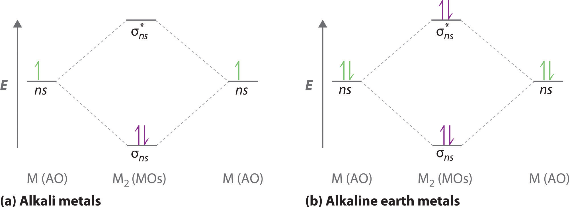
The molecular orbitals diagrams formatted for the dihydrogen species are similar to the diagrams to any homonuclear diatomic molecule with two identical alkali metal atoms (Li₂ and Cs₂, for example)

Molecular Orbital Energy-Level Diagrams for Alkali Metal and Alkaline Earth Metal Diatomic (M₂) Molecules. (a) For alkali metal diatomic molecules, the two valence electrons are enough to fill the σ_ns (bonding) level, giving a bond order of 1. (b) For alkaline earth metal diatomic molecules, the four valence electrons fill both the σ_ns (bonding) and the σ_ns* (nonbonding) levels, leading to a predicted bond order of 0. (CC BY-SA-NC; Aanonymous by request)

Atomic orbitals other than ns orbitals can also interact to form molecular orbitals. Because individual p, d, and f orbitals are not spherically symmetrical, however, we need to define a coordinate system so we know which lobes are interacting in three-dimensional space.

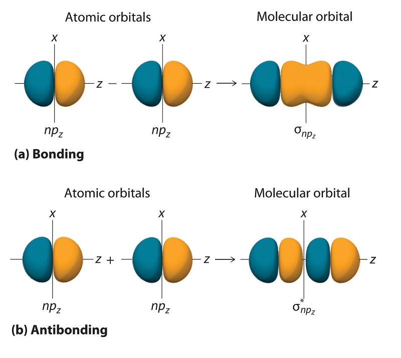
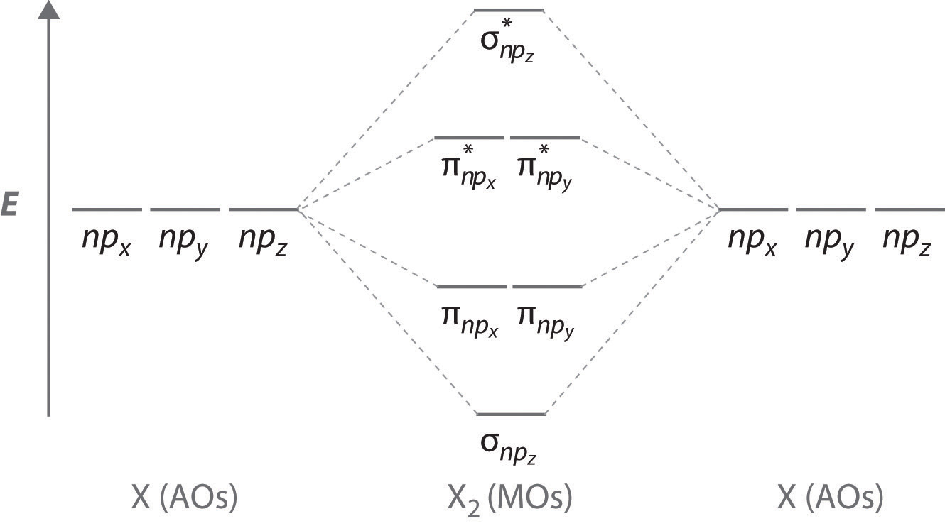
Sigma Bonding from np Orbitals

Just as with ns orbitals, we can form molecular orbitals from np orbitals by taking their mathematical sum and difference.

\[ \sigma _{np_{z}}=np_{z}\left ( A \right )-np_{z}\left ( B \right ) \label{9.7.2}\]

The other possible combination of the two np_z orbitals is the mathematical sum:

\[ \sigma _{np_{z}}=np_{z}\left ( A \right )+np_{z}\left ( B \right ) \label{9.7.3}\]

Formation of Molecular Orbitals from np_z Atomic Orbitals on Adjacent Atoms.(a) By convention, in a linear molecule or ion, the z-axis always corresponds to the internuclear axis, with +z to the right. As a result, the signs of the lobes of the np_z atomic orbitals on the two atoms alternate − + − +, from left to right. In this case, the σ (bonding) molecular orbital corresponds to the mathematical difference, in which the overlap of lobes with the same sign results in increased probability density between the nuclei. (b) In contrast, the σ* (antibonding) molecular orbital corresponds to the mathematical sum, in which the overlap of lobes with opposite signs results in a nodal plane of zero probability density perpendicular to the internuclear axis. (CC BY-SA-NC; Aanonymous by request)

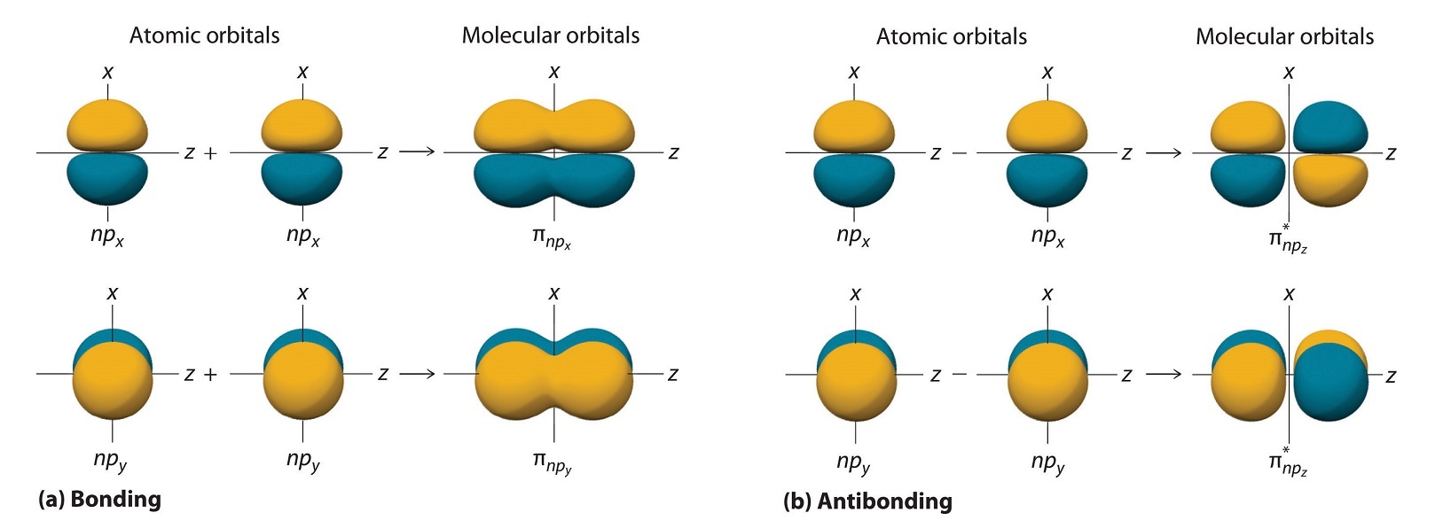
Pi bonding from np Orbitals

The remaining p orbitals on each of the two atoms, np_x and np_y, do not point directly toward each other. Instead, they are perpendicular to the internuclear axis. The np_x orbital on one atom can interact with only the np_x orbital on the other, and the np_y orbital on one atom can interact with only the np_y on the other. These interactions are side-to-side rather than the head-to-head interactions characteristic of σ orbitals. Each pair of overlapping atomic orbitals again forms two molecular orbitals: one corresponds to the arithmetic sum of the two atomic orbitals and one to the difference.

The sum of these side-to-side interactions increases the electron probability in the region above and below a line connecting the nuclei, so it is a bonding molecular orbital that is called a pi (π) orbital (a bonding molecular orbital formed from the side-to-side interactions of two or more parallel np atomic orbitals). The difference results in the overlap of orbital lobes with opposite signs, which produces a nodal plane perpendicular to the internuclear axis; hence it is an antibonding molecular orbital, called a pi star (π*) orbital An antibonding molecular orbital formed from the difference of the side-to-side interactions of two or more parallel np atomic orbitals, creating a nodal plane perpendicular to the internuclear axis..

\[ \pi _{np_{x}}=np_{x}\left ( A \right )+np_{x}\left ( B \right ) \label{9.7.4}\]

\[ \pi ^{\star }_{np_{x}}=np_{x}\left ( A \right )-np_{x}\left ( B \right ) \label{9.7.5}\]

Formation of π Molecular Orbitals from np_x and np_y Atomic Orbitals on Adjacent Atoms.(a) Because the signs of the lobes of both the np_x and the np_y atomic orbitals on adjacent atoms are the same, in both cases the mathematical sum corresponds to a π (bonding) molecular orbital. (b) In contrast, in both cases, the mathematical difference corresponds to a π* (antibonding) molecular orbital, with a nodal plane of zero probability density perpendicular to the internuclear axis. (CC BY-SA-NC; Anonymous by request)

Orbitals can Mix also

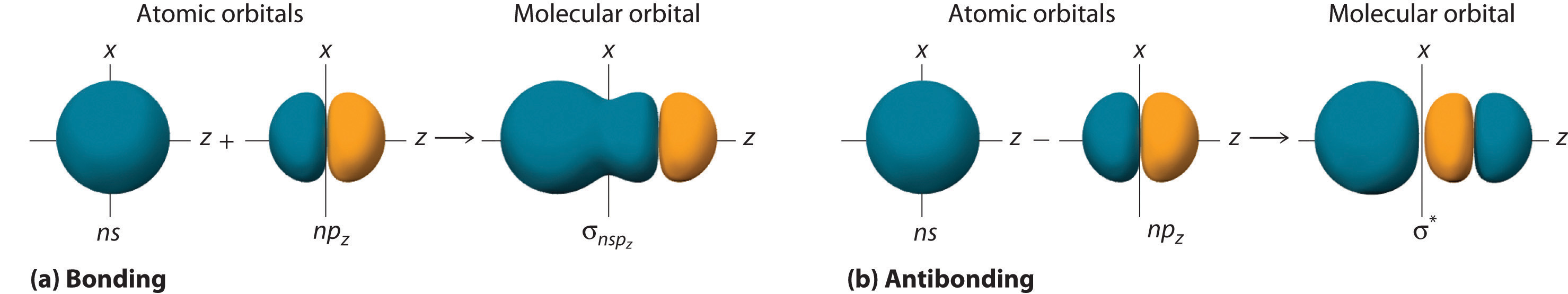
Although many combinations of atomic orbitals form molecular orbitals, we will discuss only one other interaction: an ns atomic orbital on one atom with an np_z atomic orbital on another. The sum of the two atomic wave functions (ns + np_z) produces a σ bonding molecular orbital. Their difference (ns − np_z) produces a σ* antibonding molecular orbital, which has a nodal plane of zero probability density perpendicular to the internuclear axis.

Formation of Molecular Orbitals from an ns Atomic Orbital on One Atom and an np_z Atomic Orbital on an Adjacent Atom. (a) The mathematical sum results in a σ (bonding) molecular orbital, with increased probability density between the nuclei. (b) The mathematical difference results in a σ* (antibonding) molecular orbital, with a nodal plane of zero probability density perpendicular to the internuclear axis. (CC BY-SA-NC; Anonymous by request)

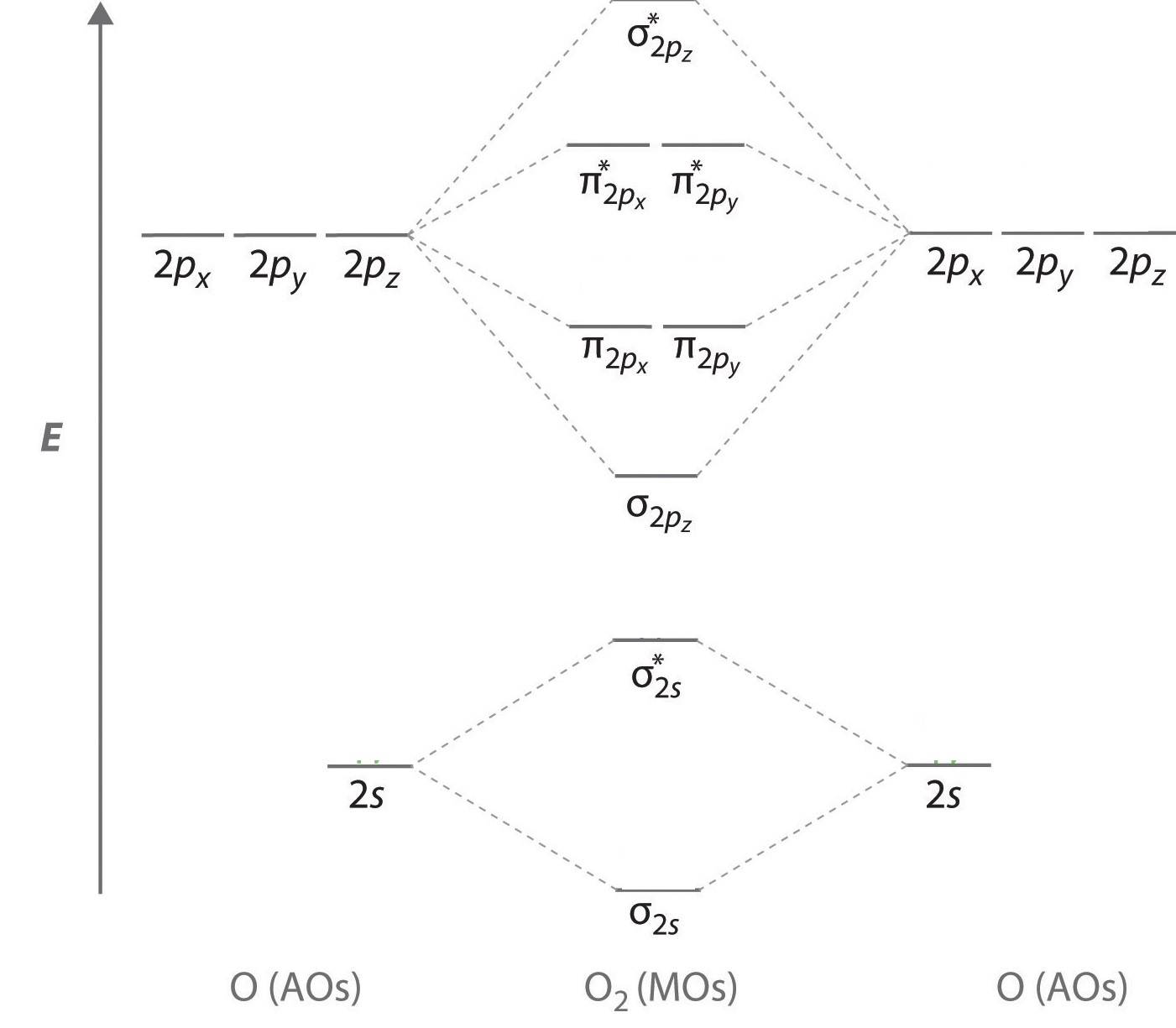
Energies of Molecular Orbitals from p atomic orbitals

Energies for Homonuclear Diatomic Molecules. The Relative Energies of the σ and π Molecular Orbitals Derived from np_x, np_y, and np_z Orbitals on Identical Adjacent Atoms. Because the two np_z orbitals point directly at each other, their orbital overlap is greater, so the difference in energy between the σ and σ* molecular orbitals is greater than the energy difference between the π and π* orbitals. (CC BY-SA-NC; Anonymous by request)

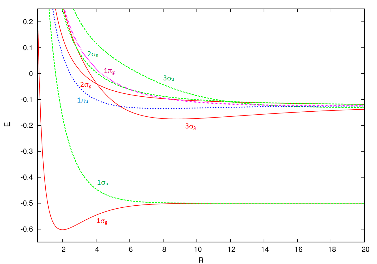
The energies of all orbitals vary with intermolecular distance (\(R\)).

Lowest energy levels of as a function of internuclear distance with internuclear repulsion included. Adapted from J. C. Slater, Quantum Theory of Matter, 2nd ed., McGraw-Hill, New York, 1968, p. 376. (Public Domain; Tonymath)

Period 2 homonuclear diatomic molecules Summary

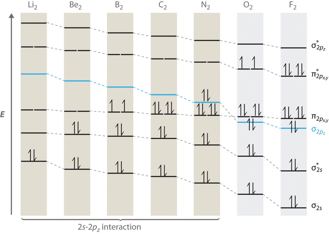
We now describe examples of systems involving period 2 homonuclear diatomic molecules, such as N₂, O₂, and F₂. When we draw a molecular orbital diagram for a molecule, there are four key points to remember:

1. The number of molecular orbitals produced is the same as the number of atomic orbitals used to create them.
2. As the overlap between two atomic orbitals increases, the difference in energy between the resulting bonding and antibonding molecular orbitals increases.
3. When two atomic orbitals combine to form a pair of molecular orbitals, the bonding molecular orbital is stabilized about as much as the antibonding molecular orbital is destabilized.
4. The interaction between atomic orbitals is greatest when they have the same energy.

The "Great Sigma-Pi Switchover"

An energy-level diagram that can be applied to two identical interacting atoms that have three np atomic orbitals each.

Molecular Orbital Energy-Level Diagrams for the Diatomic Molecules of the Period 2 Elements. Unlike earlier diagrams, only the molecular orbital energy levels for the molecules are shown here. For simplicity, the atomic orbital energy levels for the component atoms have been omitted. For Li₂ through N₂, the \( \sigma _{2p_{z}} \) orbital is higher in energy than the \( \pi _{2p_{x,y}} \) orbitals. In contrast, the \( \sigma _{2p_{z}} \) orbital is lower in energy than the \( \pi _{2p_{x,y}} \) orbitals for O₂ and F₂ due to the increase in the energy difference between the 2s and 2p atomic orbitals as the nuclear charge increases across the row. (CC BY-SA-NC; Anonymous by request)

Molecular Orbital Energy-Level Diagrams for Homonuclear Diatomic Molecules. (a) For C₂, with 8 valence electrons (4 from each C atom). This diagram shows 6 electrons in bonding orbitals and 2 in antibonding orbitals, resulting in a bond order of 2. (b) For O₂, with 12 valence electrons (6 from each O atom), there are only 2 electrons to place in the \( \left ( \pi ^{\star }_{np_{x}},\; \pi ^{\star }_{np_{y}} \right ) \) pair of orbitals. Hund’s rule dictates that one electron occupies each orbital, and their spins are parallel, giving the O₂ molecule two unpaired electrons. This diagram shows 8 electrons in bonding orbitals and 4 in antibonding orbitals, resulting in a predicted bond order of 2. (CC BY-SA-NC; Anonymous by request)

Molecular Oxygen is Paramagnetic

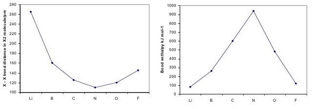
Both bond length and bond energy changes as the bond order increases and as the number of electrons shared between two atoms in a molecule increases, the bond order of a bond increases, the strength of the bond increases and the distance between nuclei decreases:

General Correlation between Bond Strength, length and order in Covalent bonds

Bond	Bond Order	Bond Enthalpy (kJ/mol)	Bond Length (Å)
\(\ce{C-C}\)	1	348	1.54
\(\ce{C=C}\)	2	614	1.34
\(\ce{C#C}\)	3	839	1.20
\(\ce{N-N}\)	1	163	1.47
\(\ce{N=N}\)	2	418	1.24
\(\ce{N#N}\)	3	941	1.10

The above trend can be observed in the first row diatomics in Figure \(\PageIndex{1}\). The bond order can be determined directly form the molecular orbital electron configurations.

\[\text{bond order} = \dfrac{\text{number of electrons in bonding MOs}- \text{number of electrons in antbonding MOs}}{2} \label{BO}\]

For diatomics, the occupations can correlate to bond length, bond energies and behavior in applied magnetic fields Figure \(\PageIndex{1}\).

Plot of bond length (left) and bond energy (right) for first row diatomics.

Example \(\PageIndex{1}\): Molecular Oxygen Species

Arrange the following four molecular oxygen species in order of increasing bond length: \(O_2^+\), \(O_2\), \(O_2^-\), and \(O_2^{2-}\).

Solution

The bond length in the oxygen species can be explained by the positions of the electrons in molecular orbital theory.

The bond order is determined from the the electron configurations via Equation \(\ref{BO}\). The electron configurations for the four species are contrasted below.

\(O_2\): 12 Electrons

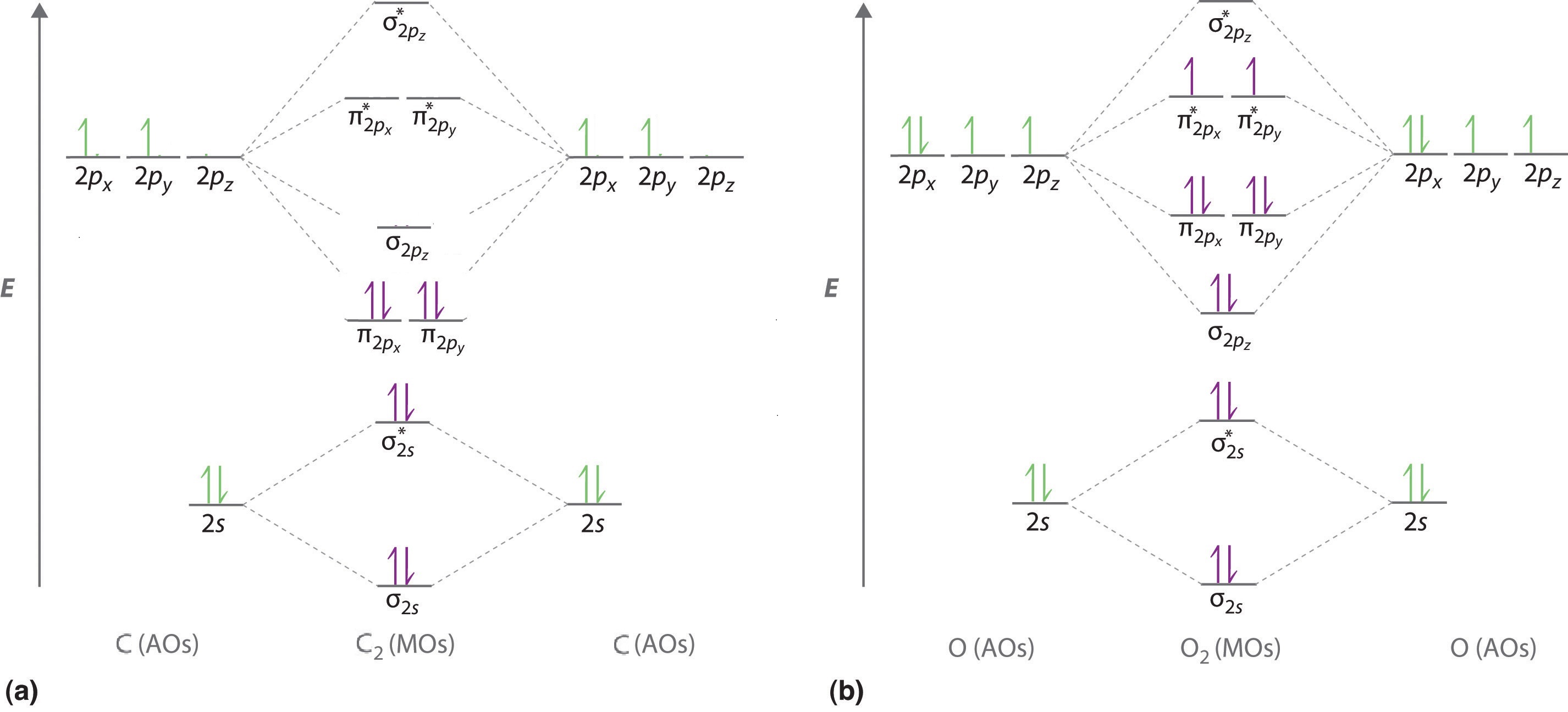
To obtain the molecular orbital energy-level diagram for O₂, we need to place 12 valence electrons (6 from each O atom) in the energy-level diagram shown in Figure \(\PageIndex{1}\). We again fill the orbitals according to Hund’s rules and the Pauli principle, beginning with the orbital that is lowest in energy. Two electrons each are needed to fill the σ_2s and σ_2s* orbitals, two more to fill the \( \sigma _{2p_{z}} \) orbital, and 4 to fill the degenerate \( \pi _{2p_{x}}^{\star } \) and \( \pi _{2p_{y}}^{\star } \) orbitals. According to Hund’s first rule, the last 2 electrons must be placed in separate \(π^*\) orbitals with their spins parallel, giving a multiplicity of 3 (a triplet state) with two unpaired electrons. This leads to a predicted bond order of

\[\dfrac{8 − 4}{2} = 2 \nonumber\]

which corresponds to a double bond, in agreement with experimental data: the O–O bond length is 120.7 pm, and the bond energy is 498.4 kJ/mol at 298 K.

\[σ_{1s}^2 {σ^*_{1s}}^2 σ_{2s}^2 {σ^*_{2s}}^2 σ_{2p}^2 π_{2p_y}^2 {π^*_{2p_y}}^2 π_{2p_x}^1 {π^*_{2p_y}}^1 \nonumber \]

From the equation above the bond order for \(O_2\) is 2 (i.e., a double bond).

\(O_2^{+}\): 11 Electrons

\[σ_{1s}^2 {σ^*_{1s}}^2 σ_{2s}^2 {σ^*_{2s}}^2 σ_{2p}^2 π_{2p_y}^2 {π^*_{2p_y}}^2 π_{2p_x}^1 {π^*_{2p_y}}^0 \nonumber \]

From the equation above the bond order for \(O_2^{+}\) is 2.5.

\(O_2^{-}\): 13 Electrons

\[σ_{1s}^2 {σ^*_{1s}}^2 σ_{2s}^2 {σ^*_{2s}}^2 σ_{2p}^2 π_{2p_y}^2 {π^*_{2p_y}}^2 π_{2p_x}^1 {π^*_{2p_y}}^2 \nonumber \]

From the equation above the bond order for \(O_2^{-}\) is 1.5.

\(O_2^{2-}\): 14 Electrons

\[σ_{1s}^2 {σ^*_{1s}}^2 σ_{2s}^2 {σ^*_{2s}}^2 σ_{2p}^2 π_{2p_y}^2 {π^*_{2p_y}}^2 π_{2p_x}^2 {π^*_{2p_y}}^2 \nonumber \]

From the equation above the bond order for \(O_2^{2-}\) is 1.

The bond order decreases and the bond length increases in the order. The predicted order of increasing bondlength then is \(O_2^+\) < \(O_2\) < \(O_2^-\) < \(O_2^{2-}\). This trend is confirmed experimentally with \(O_2^+\) (112.2 pm), \(O_2\) (121 pm), \(O_2^-\) (128 pm) and \(O_2^{2-}\) (149 pm).

Liquid O₂ Suspended between the Poles of a Magnet. Because the O₂ molecule has two unpaired electrons, it is paramagnetic. Consequently, it is attracted into a magnetic field, which allows it to remain suspended between the poles of a powerful magnet until it evaporates.