
17: Hydrogen-like Solutions
- Page ID
- 39852
\( \newcommand{\vecs}[1]{\overset { \scriptstyle \rightharpoonup} {\mathbf{#1}} } \)
\( \newcommand{\vecd}[1]{\overset{-\!-\!\rightharpoonup}{\vphantom{a}\smash {#1}}} \)
\( \newcommand{\id}{\mathrm{id}}\) \( \newcommand{\Span}{\mathrm{span}}\)
( \newcommand{\kernel}{\mathrm{null}\,}\) \( \newcommand{\range}{\mathrm{range}\,}\)
\( \newcommand{\RealPart}{\mathrm{Re}}\) \( \newcommand{\ImaginaryPart}{\mathrm{Im}}\)
\( \newcommand{\Argument}{\mathrm{Arg}}\) \( \newcommand{\norm}[1]{\| #1 \|}\)
\( \newcommand{\inner}[2]{\langle #1, #2 \rangle}\)
\( \newcommand{\Span}{\mathrm{span}}\)
\( \newcommand{\id}{\mathrm{id}}\)
\( \newcommand{\Span}{\mathrm{span}}\)
\( \newcommand{\kernel}{\mathrm{null}\,}\)
\( \newcommand{\range}{\mathrm{range}\,}\)
\( \newcommand{\RealPart}{\mathrm{Re}}\)
\( \newcommand{\ImaginaryPart}{\mathrm{Im}}\)
\( \newcommand{\Argument}{\mathrm{Arg}}\)
\( \newcommand{\norm}[1]{\| #1 \|}\)
\( \newcommand{\inner}[2]{\langle #1, #2 \rangle}\)
\( \newcommand{\Span}{\mathrm{span}}\) \( \newcommand{\AA}{\unicode[.8,0]{x212B}}\)
\( \newcommand{\vectorA}[1]{\vec{#1}} % arrow\)
\( \newcommand{\vectorAt}[1]{\vec{\text{#1}}} % arrow\)
\( \newcommand{\vectorB}[1]{\overset { \scriptstyle \rightharpoonup} {\mathbf{#1}} } \)
\( \newcommand{\vectorC}[1]{\textbf{#1}} \)
\( \newcommand{\vectorD}[1]{\overrightarrow{#1}} \)
\( \newcommand{\vectorDt}[1]{\overrightarrow{\text{#1}}} \)
\( \newcommand{\vectE}[1]{\overset{-\!-\!\rightharpoonup}{\vphantom{a}\smash{\mathbf {#1}}}} \)
\( \newcommand{\vecs}[1]{\overset { \scriptstyle \rightharpoonup} {\mathbf{#1}} } \)
\( \newcommand{\vecd}[1]{\overset{-\!-\!\rightharpoonup}{\vphantom{a}\smash {#1}}} \)
\(\newcommand{\avec}{\mathbf a}\) \(\newcommand{\bvec}{\mathbf b}\) \(\newcommand{\cvec}{\mathbf c}\) \(\newcommand{\dvec}{\mathbf d}\) \(\newcommand{\dtil}{\widetilde{\mathbf d}}\) \(\newcommand{\evec}{\mathbf e}\) \(\newcommand{\fvec}{\mathbf f}\) \(\newcommand{\nvec}{\mathbf n}\) \(\newcommand{\pvec}{\mathbf p}\) \(\newcommand{\qvec}{\mathbf q}\) \(\newcommand{\svec}{\mathbf s}\) \(\newcommand{\tvec}{\mathbf t}\) \(\newcommand{\uvec}{\mathbf u}\) \(\newcommand{\vvec}{\mathbf v}\) \(\newcommand{\wvec}{\mathbf w}\) \(\newcommand{\xvec}{\mathbf x}\) \(\newcommand{\yvec}{\mathbf y}\) \(\newcommand{\zvec}{\mathbf z}\) \(\newcommand{\rvec}{\mathbf r}\) \(\newcommand{\mvec}{\mathbf m}\) \(\newcommand{\zerovec}{\mathbf 0}\) \(\newcommand{\onevec}{\mathbf 1}\) \(\newcommand{\real}{\mathbb R}\) \(\newcommand{\twovec}[2]{\left[\begin{array}{r}#1 \\ #2 \end{array}\right]}\) \(\newcommand{\ctwovec}[2]{\left[\begin{array}{c}#1 \\ #2 \end{array}\right]}\) \(\newcommand{\threevec}[3]{\left[\begin{array}{r}#1 \\ #2 \\ #3 \end{array}\right]}\) \(\newcommand{\cthreevec}[3]{\left[\begin{array}{c}#1 \\ #2 \\ #3 \end{array}\right]}\) \(\newcommand{\fourvec}[4]{\left[\begin{array}{r}#1 \\ #2 \\ #3 \\ #4 \end{array}\right]}\) \(\newcommand{\cfourvec}[4]{\left[\begin{array}{c}#1 \\ #2 \\ #3 \\ #4 \end{array}\right]}\) \(\newcommand{\fivevec}[5]{\left[\begin{array}{r}#1 \\ #2 \\ #3 \\ #4 \\ #5 \\ \end{array}\right]}\) \(\newcommand{\cfivevec}[5]{\left[\begin{array}{c}#1 \\ #2 \\ #3 \\ #4 \\ #5 \\ \end{array}\right]}\) \(\newcommand{\mattwo}[4]{\left[\begin{array}{rr}#1 \amp #2 \\ #3 \amp #4 \\ \end{array}\right]}\) \(\newcommand{\laspan}[1]{\text{Span}\{#1\}}\) \(\newcommand{\bcal}{\cal B}\) \(\newcommand{\ccal}{\cal C}\) \(\newcommand{\scal}{\cal S}\) \(\newcommand{\wcal}{\cal W}\) \(\newcommand{\ecal}{\cal E}\) \(\newcommand{\coords}[2]{\left\{#1\right\}_{#2}}\) \(\newcommand{\gray}[1]{\color{gray}{#1}}\) \(\newcommand{\lgray}[1]{\color{lightgray}{#1}}\) \(\newcommand{\rank}{\operatorname{rank}}\) \(\newcommand{\row}{\text{Row}}\) \(\newcommand{\col}{\text{Col}}\) \(\renewcommand{\row}{\text{Row}}\) \(\newcommand{\nul}{\text{Nul}}\) \(\newcommand{\var}{\text{Var}}\) \(\newcommand{\corr}{\text{corr}}\) \(\newcommand{\len}[1]{\left|#1\right|}\) \(\newcommand{\bbar}{\overline{\bvec}}\) \(\newcommand{\bhat}{\widehat{\bvec}}\) \(\newcommand{\bperp}{\bvec^\perp}\) \(\newcommand{\xhat}{\widehat{\xvec}}\) \(\newcommand{\vhat}{\widehat{\vvec}}\) \(\newcommand{\uhat}{\widehat{\uvec}}\) \(\newcommand{\what}{\widehat{\wvec}}\) \(\newcommand{\Sighat}{\widehat{\Sigma}}\) \(\newcommand{\lt}{<}\) \(\newcommand{\gt}{>}\) \(\newcommand{\amp}{&}\) \(\definecolor{fillinmathshade}{gray}{0.9}\)Last lecture we completed the discussion of Rigid Rotors within the context of microwave spectroscopy (a topic of Worksheet 4B: Rotational Spectroscopy). We introduce the hydrogen atom (the most important model and real system for quantum chemistry), by defining the potential, Hamiltonian and Schrodinger equation. We argued the solution of the Schodinger equation involves a radial component and an angular component. The latter is just the spherical harmonics derived in the rigid rotor system previously. We ended lecture on the radial component which is a function of four terms: A normalization constant, associated Laguerre polynomial, a nodal function, and an exponential decay. We also discussed that the energy is a function of only one quantum number and that there is a degeneracy of the wavefunctions.
Java simulation of particles in boxes :https://phet.colorado.edu/en/simulation/bound-states
The Eigenvalue Problem for the Hydrogen Atom
Step 1: Define the Schrödinger Equation for the problem
For the Hydrogen atom, the potential energy is given by the Coulombic potential, which is
\[\color{red}V(r) = -\dfrac {e^2}{4\pi \epsilon_0 r}\]
With every quantum eigenvalue problem, we define the Hamiltonian as such:
\[\hat {H} = T + V\]
The potential is defined above and the Kinetic energy is given by
\[T = -\dfrac {\hbar^2}{2m_e} \bigtriangledown^2\]
The Hamiltonian for the Hydrogen atom becomes
\[\hat {H} = -\dfrac {\hbar^2}{2m_e}\bigtriangledown^2 - \dfrac {e^2}{4\pi \epsilon_0 r}\label {1}\]
and since the potential has no time-dependence, we can se the time independent Schrödinger Equation
\[\hat {H} | \psi (x,y,z) \rangle = E | \psi (x,y,z) \rangle \]
Step 2: Solve the Schrödinger Equation for the problem
The potential has a spherical symmetry (i.e., depends only on \(r\) and not typically in terms of \(x\), \(y\) and \(z\)), so switching to spherical coordinates is useful. The new eigenvalue problem is
\[ \begin{align} \hat {H}\psi(r,\theta,\phi) &= -\dfrac {\hbar^2}{2m_e} \left [\dfrac {1}{r^2} \dfrac {d}{d r} \left(r^2 \dfrac {d \psi(r,\theta,\phi)}{d r}\right) + \dfrac {1}{r^2 \sin(\theta)} \dfrac {d}{d \theta} \left(\sin(\theta) \dfrac {d \psi(r,\theta,\phi)}{d \theta}\right) + \dfrac {1}{r^2 \sin^2(\theta)} \dfrac {d^2 \psi(r,\theta,\phi)}{d \phi^2} \right] - \dfrac {e^2}{4\pi\epsilon_0 r} \psi(r,\theta,\phi) \label{eq2} \\[4pt] &= E\psi (r,\theta,\phi) \label{2} \end{align}\]
Multiplying Equation \ref{eq2} by \(2m_e r^2\) and moving \(E\) to the left side gives
\[\hbar^2 \left(\dfrac {d}{d r} r^2 \dfrac {d \psi(r,\theta,\phi) }{d r}\right) - \hbar^2 \left[\dfrac {1}{\sin (\theta)} \left(\dfrac {d}{d \theta} \sin (\theta) \dfrac {d \psi(r,\theta,\phi) }{d \theta}\right) + \dfrac {1}{\sin^2 (\theta)} \dfrac {d^2 \psi(r,\theta,\phi) }{d \phi^2} \right] - 2m_e r^2 \left [\dfrac {e^2}{4\pi\epsilon_0 r} + E \right] \psi (r,\theta,\phi) = 0 \label {3}\]
Although Equation \(\ref{3}\) is a complex equation, it can be simplified by using the definition of the \(\hat{L}^2\) operator,
\[\hat{L^2} = - \hbar^2 \left [\dfrac {1}{\sin (\theta)} \left(\dfrac {d}{d \theta} \sin (\theta\right) \dfrac {d \psi}{d \theta}) + \dfrac {1}{\sin^2 (\theta)} \dfrac {d^2 \psi}{d \phi^2}\right] \label{ 4a}\]
where
\[\hat {L^2} Y_{\ell}^{m} = \hbar^2 \ell(\ell + 1) Y_{\ell}^{m} \label{4c}\]
We then can use a separation of variables argument for the radial and angular components to postulate a general solution
\[ \color{red} \psi(r,\theta,\phi) = R(r)Y_{\ell}^{m}(\theta,\phi) \label{4b}\]
Using these three equations for Equation \(\ref{3}\) gives
\[-\dfrac {\hbar^2}{2m_e r^2} \dfrac {d}{d r} \left(r^2 \dfrac {d R(r)}{d r}\right) + \left[\dfrac {\hbar^2 \ell(\ell+1)}{2m_e r^2} - \dfrac{e^2}{4\pi\epsilon_0 r} - E \right] R(r) = 0 \label {5}\]
A solution for \(R(r)\) can be found with a quantum number \(n\), and then \(E_n\) is solved as
\[ \color{red} E_n = -\dfrac {m_e e^4}{8\epsilon_0^2 h^2 n^2}\label{6}\]
with \(n=1,2,3 ...\infty\)
Step 3: Do something with the Eigenstates and associated energies
Let's talk about the solutions first.
Ranges of the Three Quantum Numbers
In solving these types of differential equations, there are limits on \(\ell\) and \(m_{\ell}\), but not \(n\).
- \(n = 1, 2, 3, ...\infty\)
- \(\ell = 0, 1, 2, ... (n-1)\)
- \(m_{\ell} = 0, \pm 1, \pm 2, ... \pm \ell\)
Energy
The motion of the electron in the hydrogen atom is not free. The electron is bound to the atom by the attractive force of the nucleus and consequently quantum mechanics predicts that the total energy of the electron is quantized. The expression for the energy is:
\[E_n =\dfrac{-2 \pi^2 m e^4Z^2}{n^2h^2} \label{17.1}\]
with \(n = 1,2,3,4...\)
where \(m\) is the mass of the electron, \(e\) is the magnitude of the electronic charge, \(n\) is a quantum number, \(h\) is Planck's constant and \(Z\) is the atomic number (the number of positive charges in the nucleus).
Equation \(\ref{17.1}\) is often reexpressed as
\[E_n = \dfrac{Z^2 E_h}{2 n^2} \label{17.1A}\]
where \(E_h\) is the Hartree energy (27.211 eV). Equation \(\ref{17.1}\) applies to any one-electron atom or ion. For example, He+ is a one-electron system for which Z = 2. We can again construct an energy level diagram listing the allowed energy values (Figure \(\PageIndex{1}\)).

These are obtained by substituting all possible values of \(n\) into Equation \(\ref{17.1}\). As in our previous example, we shall represent all the constants that appear in the expression for \(E_n\) by the Rydberg constant \(R\) and we shall set \(Z = 1\), i.e., consider only the hydrogen atom.
\[ E_n = \dfrac{-R}{n^2} \label{17.2}\]
with \(n = 1,2,3,4,...\).
How much energy (in eV) is required to remove an electron from each of the following orbitals in a hydrogen atom:
- 2p
- 6p
- Approach
-
The removal of an electron from a hydrogen atom is akin to moving an electron from energy state \(n\) to a distance infinity. The energy required for this is called the ionization energy, which is given by Equation \ref{17.1A} for the energy of a one-electron atom (i.e., any hydrogenic atom)
\[E_n = \dfrac{Z^2 E_h}{2 n^2} \nonumber\]
where \(E_h\) is the Hartree energy and \(Z\) is the atomic charge (for hydrogen \(Z=1\)).
- Answer a
-
\[E_2 = \dfrac{(1)^2 (27.211\;eV)}{2 (2)^2} = 3.40\;eV \nonumber\]
- Answer b
-
\[E_6 = \dfrac{(1)^2 (27.211\;eV)}{2 (6)^2} = 1.51378\;eV \nonumber\]
- Comment
-
As expected from Figure \(\PageIndex{1}\), the 6p election is less stabilized (i.e., higher in energy) than the 2p electron and hence requires less energy to extract.
Orthonormality of the Eigenstates
The normalization condition for the hydrogen atomic wavefunction is given by
\[ \langle \psi_{n' \ell' m'_\ell} | \psi_{n \ell m_\ell} \rangle = \delta_{nn'} \delta_{\ell\ell'} \delta_{m_\ell m'_\ell}\label{6b}\]
where each \(n\), \(\ell\), \(m_\ell\) value correspond to a specific wavefunction.
And the Kronecker delta is defined as
\[\delta _{mn}\equiv \begin{bmatrix}1\; if\; m=n\\ 0\; if\; m\neq n\end{bmatrix}\label{3.5.21}\]
The specific eigenstates for the hydrogen atom wavefunctions are
\[ | \psi_{n \ell m_\ell}(r,\theta,\phi) \rangle = |R(r) Y_{\ell}^{m}(\theta,\phi) \rangle \label{7b}\]
For example, \(| \psi_{100} \rangle \) corresponds to a wavefunction with \(n=1, \ell=0, m_{\ell} = 0\). This is the 1s orbital and thus \(\psi_{100}\) can also be referred to as \(\psi_{1s}\). With the same reasoning, \(| \psi_{210} \rangle\) refers to \(\psi_{2p_z}\)
Equation \ref{6b} in integral formulation is
\[\int_0^{\infty} \int_0^{\pi} \int_0^{2\pi} \psi^*_{n' \ell' m'_\ell} \psi_{n \ell m_\ell} \underbrace{r^2 \sin(\theta)}_{Jacobian} \, d\phi\, d\theta\,dr = \delta_{nn'} \delta_{\ell\ell'} \delta_{m_\ell m'_\ell}\label{7a}\]
While every eigenstate has a specific set of quantum numbers associated with it (like \(\psi_{1s}\) with \(n=1, \ell=0, m_{\ell} = 0\)), this does NOT always apply to the orbitals introduced in general chemistry. As discussed later, some orbitals are formed as a combination of wavefunctions (since they are degenerate) so that we cannot ascribe one set of three quantum numbers to them. This will be discussed later.
Angular Part
From our work on the rigid rotor, we know that the eigenfunctions of the angular momentum operator are the Spherical Harmonic functions (Table M4), \(Y (\theta ,\phi )\),
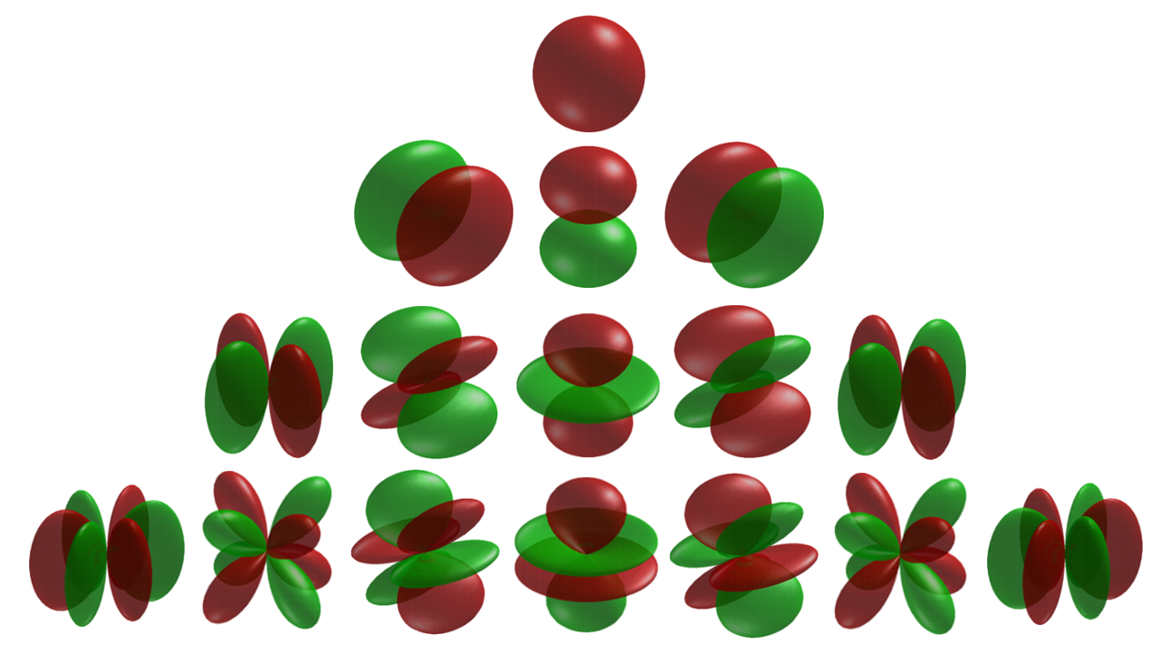
Radial Part of the Wavefunction
The Spherical Harmonic functions provide information about where the electron is around the proton, and the radial function \(R(r)\) describes how far the electron is away from the proton. The \(R(r)\) functions that solve the radial differential equation, are products of the associated Laguerre polynomials times the exponential factor, multiplied by a normalization factor \((N_{n,l})\) and \(\left (\dfrac {r}{a_0} \right)^l\).
\[ \color{red} R (r) = \underbrace{N_{n,l} \left ( \dfrac {r}{a_0} \right ) ^l}_{\text{Normalization}} \times \overbrace{L_{n,l} (r)}^{\text{Laguerre Poly}} \times \underbrace{e^{-\frac {r}{n {a_0}}}}_{\text{exponential}} \label {6.1.17}\]
The decreasing exponential term overpowers the increasing polynomial term so that the overall wavefunction exhibits the desired approach to zero at large values of \(r\). The first six radial functions are provided in Table below. Note that the functions in the table exhibit a dependence on \(Z\), the atomic number of the nucleus.
|
|
|
|
|---|---|---|
| 1 | 0 | \(2 \left( \dfrac{Z}{a_o} \right)^{3/2} e^{ -Zr/a_o}\) |
| 2 | 0 | \(\dfrac{1}{2\sqrt{2}} \left( \dfrac{Z}{a_o} \right)^{3/2}\left [2-\dfrac{Zr}{a_o} \right]e^{ -Zr/2a_o}\) |
| 2 | 1 | \(\dfrac{1}{2\sqrt{6}} \left( \dfrac{Z}{a_o} \right)^{3/2}\left [\dfrac{Zr}{a_o} \right] e^{ -Zr/2a_o}\) |
| 3 | 0 | \(\dfrac{2}{81 \sqrt{3}} \left( \dfrac{Z}{a_o} \right)^{3/2}\left [27 -18 \dfrac{Zr}{a_o} +2 \left( \dfrac{Zr}{a_o}\right)^2 \right] e^{ -Zr/3a_o}\) |
| 3 | 1 | \(\dfrac{4}{81 \sqrt{6}} \left( \dfrac{Z}{a_o} \right)^{3/2}\left [6 \dfrac{Zr}{a_o} - \left( \dfrac{Zr}{a_o}\right)^2 \right] e^{ -Zr/3a_o}\) |
| 3 | 2 | \(\dfrac{4}{81 \sqrt{30}} \left( \dfrac{Z}{a_o} \right)^{3/2} \left ( \dfrac{Zr}{a_o} \right)^2 e^{ -Zr/3a_o}\) |
Java simulation of particles in boxes :https://phet.colorado.edu/en/simulation/bound-states
Laguerre polynomials
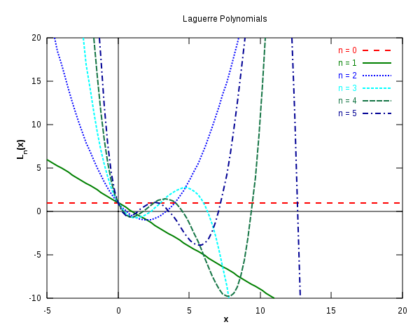
The first six Laguerre polynomials. from Wikipedia.
The constraint that \(n\) be greater than or equal to \(l +1\) also turns out to quantize the energy, producing the same quantized expression for hydrogen atom energy levels that was obtained from the Bohr model of the hydrogen atom discussed in Chapter 2.
\[ E_n = - \dfrac {m_e e^4}{8 \epsilon ^2_0 h^2 n^2} \]
It is interesting to compare the results obtained by solving the Schrödinger equation with Bohr’s model of the hydrogen atom. There are several ways in which the Schrödinger model and Bohr model differ.
- First, and perhaps most strikingly, the Schrödinger model does not produce well-defined orbits for the electron. The wavefunctions only give us the probability for the electron to be at various directions and distances from the proton.
- Second, the quantization of angular momentum is different from that proposed by Bohr. Bohr proposed that the angular momentum is quantized in integer units of \(\hbar\), while the Schrödinger model leads to an angular momentum of \( \sqrt{(l (l +1) \hbar ^2} \).
- Third, the quantum numbers appear naturally during solution of the Schrödinger equation while Bohr had to postulate the existence of quantized energy states. Although more complex, the Schrödinger model leads to a better correspondence between theory and experiment over a range of applications that was not possible for the Bohr model.
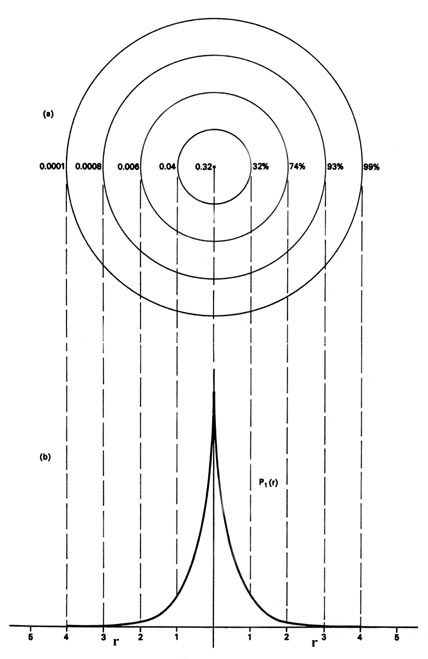
Methods for separately examining the radial portions of atomic orbitals provide useful information about the distribution of charge density within the orbitals.
We could also represent the distribution of negative charge in the hydrogen atom in the manner used previously for the electron confined to move on a plane (Figure \(\PageIndex{1}\)), by displaying the charge density in a plane by means of a contour map. Imagine a plane through the atom including the nucleus. The density is calculated at every point in this plane. All points having the same value for the electron density in this plane are joined by a contour line (Figure \(\PageIndex{3}\)). Since the electron density depends only on r, the distance from the nucleus, and not on the direction in space, the contours will be circular. A contour map is useful as it indicates the "shape" of the density distribution.
| \(n\) |
\(\ell\) |
\(m_\ell\) | Eigenstates |
|---|---|---|---|
| \(n=1\) | \(\ell=0\) | \(m=0\) | \(\psi_{100} = \dfrac {1}{\sqrt {\pi}} \left(\dfrac {Z}{a_0}\right)^{\frac {3}{2}} e^{-\rho}\) |
| \(n=2\) | \(\ell=0\) | \(m=0\) | \(\psi_{200} = \dfrac {1}{\sqrt {32\pi}} \left(\dfrac {Z}{a_0}\right)^{\frac {3}{2}} (2-\rho)e^{\dfrac {-\rho}{2}}\) |
| \(\ell=1\) | \(m=0\) | \(\psi_{210} = \dfrac {1}{\sqrt {32\pi}} \left(\dfrac {Z}{a_0}\right)^{\frac {3}{2}} \rho e^{-\rho/2} \cos(\theta)\) | |
| \(\ell=1\) | \(m=\pm 1\) | \(\psi_{21\pm\ 1} = \dfrac {1}{\sqrt {64\pi}} \left(\dfrac {Z}{a_0}\right)^{\dfrac {3}{2}} \rho e^{-\rho/2} \sin(\theta) e^{\pm\ i\phi}\) | |
| \(n=3\) | \(\ell=0\) | \(m=0\) | \(\psi_{300} = \dfrac {1}{81\sqrt {3\pi}} \left(\dfrac {Z}{a_0}\right)^{\frac {3}{2}} (27-18\rho +2\rho^2)e^{-\rho/3}\) |
| \(\ell=1\) | \(m=0\) | \(\psi_{310} = \dfrac{1}{81} \sqrt {\dfrac {2}{\pi}} \left(\dfrac {Z}{a_0}\right)^{\dfrac {3}{2}} (6\rho - \rho^2)e^{-\rho/3} \cos(\theta)\) | |
| \(\ell=1\) | \(m=\pm 1\) | \(\psi_{31\pm\ 1} = \dfrac {1}{81\sqrt {\pi}} \left(\dfrac {Z}{a_0}\right)^{\frac {3}{2}} (6\rho - \rho^2)e^{-\rho/3} \sin(\theta)e^{\pm\ i \phi}\) | |
| \(\ell=2\) | \(m=0\) | \(\psi_{320} = \dfrac {1}{81\sqrt {6\pi}} \left(\dfrac {Z}{a_0}\right)^{\frac {3}{2}} \rho^2 e^{-\rho/3}(3\cos^2(\theta) -1)\) | |
| \(\ell=2\) | \(m=\pm 1\) | \(\psi_{32\pm\ 1} = \dfrac {1}{81\sqrt {\pi}} \left(\dfrac {Z}{a_0}\right)^{\frac {3}{2}} \rho^2 e^{-\rho/3} \sin(\theta)\cos(\theta)e^{\pm\ i \phi}\) | |
| \(\ell=2\) | \(m=\pm 2\) | \(\psi_{32\pm\ 2} = \dfrac {1}{162\sqrt {\pi}} \left(\dfrac {Z}{a_0}\right)^{\frac {3}{2}} \rho^2 e^{-\rho/3}{\sin}^2(\theta)e^{\pm\ 2i\phi}\) |