15: 3D Rotations and Microwave Spectroscopy

Lecture 14

Last lecture continued the discussion of symmetry (and direct product tables for odd/even functions). We showed the quantum Harmonic Oscillator wavefunctions alternate between even and odd because of the Hermite polynomial component. This maps into the transition moment integral to predict that only transition in the IR between adjacent wavefunctions will be allowed (i.e., no harmonics will be observed). We demonstrated that this is not what is experimentally observed since overtones can be weakly observed, which means the harmonic oscillator is an approximation of a true bond. We discussed the Taylor expansion of an arbitrary potential results in the HO as the first meaningful term and higher order terms are call anharmonic terms. We introduced the Morse oscillator which is a functional form that far better approximates the true potential of vibration. The second part of the lecture introduced rotations, first by motivating classical rotation, then 2D quantum (one quantum number) and finally 3D rotation (two quantum numbers). We continue with that discussion here.

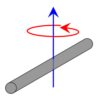
Classical Rotation of a Diatomic Molecule

Angular momentum can be considered a rotational analog of linear momentum. Thus, where linear momentum is proportional to mass \(m\) and linear speed \(v\).

\[ p =mv \tag{linear momentum}\]

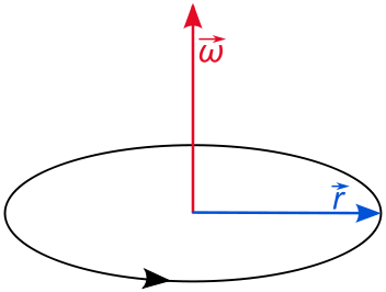
angular momentum \(J\) is proportional to moment of inertia \(I\) and angular speed \(\omega\).

The moment of inertia \(I\) of a rigid body determines the torque needed for a desired angular acceleration about a rotational axis.

For a diatomic

\[I= \mu r^2 \label{moment}\]

• where \(\mu\) is the reduced mass discussed previously \[\mu= \dfrac{m_1m_2}{m_1+m_2} \tag{reduced mass}\]
• \(r\) is the bond length (remember no vibration occurs in rigid rotors, so this is the equilibrium bond length)

The angular momentum perpendicular to the rotational motion \(L_z\) is

\[L_z = mvr \tag{angular momentum}\]

with energies

\[E=\dfrac{L_z^2}{2I} \tag{classical energy of a rigid rotor}\]

The angular velocity describes the speed of rotation and the orientation of the instantaneous axis about which the rotation occurs. The direction of the angular velocity pseudovector will be along the axis of rotation; in this case (counter-clockwise rotation) the vector points up. (CC BY-SA 3.0; dnet via Wikipedia)

2D Quantum Rigid Rotor (rotation in a single plane)

The angular momentum of a rigid rotor is

\[L_z = pr\]

Using the de Broglie relation \(p = \dfrac{h}{\lambda}\) we also have a condition for quantization of angular motion

\[L_z= \dfrac{hr}{\lambda}\]

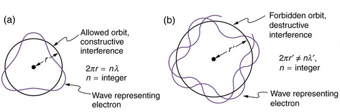
The wavelength must be a whole number fraction of the circumference for the ends to match after each circuit (remember the Bohr atom discussion).

(A) Waves on a string have a wavelength related to the length of the string, allowing them to interfere constructively. (B) If we imagine the string bent into a closed circle, we get a rough idea of how electrons in circular orbits can interfere constructively. (c) If the wavelength does not fit into the circumference, the electron interferes destructively; it cannot exist in such an orbit. from Boundless.

Hence, the condition

\[\dfrac{2\pi r}{m} =\lambda\]

combined with the deBroglie relation leads to a quantized expression of angular momentum

\[L_z=m\hbar \tag{quantization of angular momentum}\]

In these equations \(m\) is a quantum number that originates from the boundary condition of the system (just like \(n\) in the particle-in-a-box originates from that system's boundary conditions). The Hamiltonian for a rigid rotor is then

\[ - \dfrac{\hbar^2}{2I} \dfrac{\partial ^2 }{\partial \phi^2} \label{RR Hamiltonian} \]

The corresponding wavefunctions are:

\[ \color{red} |\Phi_m \rangle = \sqrt{\dfrac{1}{2\pi}} e ^{im\phi} \label{eigenstates of a 2D RR}\]

with the constraint that:

\[ m =\pm \dfrac{\sqrt{2IE}}{\hbar} \label{eigenenergies of a 2D RR}\]

The angular momentum is quantized

\[\color{red} L_z = m\hbar\]

and the energy is also quantized:

\[ \color{red} E = \dfrac{L_z^2}{2I} = \dfrac{m^2\hbar^2}{2I} \label{Energies are quantized}\]

we find that the quantum numbers for 2D rotation are

\[ \color{red} m = 0, \pm 1, \pm 2, ... \pm \infty \label{quantum number for 2D RR}\]

Properties and Notes about 2D rigid Rotor

• Solutions of the 2D Rigid Rotor rotational Hamiltonian are sine and cosine functions just like the particle in a box.
• Here the boundary condition is imposed by the circle and the fact that the wavefunction must not interfere with itself.
• This model is similar to condition in the Bohr model of the atom
• The energy and wavefunctions are dependent on the quantum number \(m\) that varies from \(-\infty\) to \(+\infty\).
• There is no zero point energy for rotation; this is similar to translation of a free particle. Zero point energies are encountered when a particle if bound like in a particle in a box or a harmonic oscillator).

3D Quantum Rigid Rotor

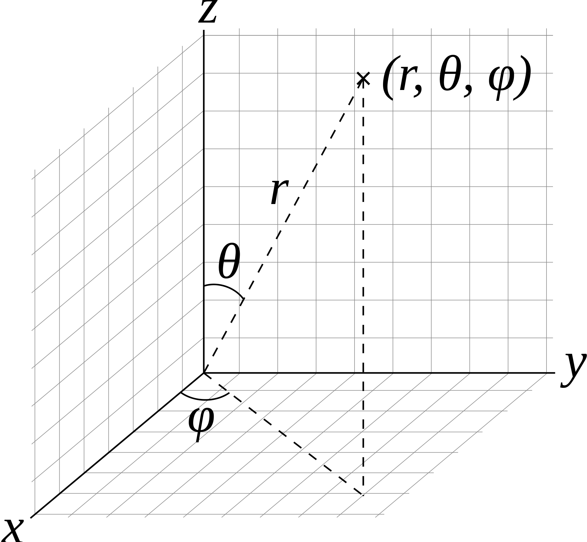
Read The Energy Levels of a Rigid Rotator for more complete derivation! For the rigid rotator, we are switching from Cartesian coordinates \(x,y,z\) to Spherical coordinates \(r,\theta, \phi\), and the variables \(r\) and \(\ell\) or \(r_o\) or \(r_{eq}\) can be used interchangeably, as they both refer to the bond distance.

Spherical coordinates (r, θ, φ) as often used in mathematics: radial distance r, azimuthal angle θ, and polar angle φ. The meanings of θ and φ have been swapped compared to the physics convention. of Wikipedia.

All bond length changes are put in the Harmonic Oscillator problem. This allows for the separation of variables between \(\theta\) and \(\phi\), as \(r\) is part of the Harmonic Oscillator. In Cartesian Coordinates,

\[\hat{T} = \hat{H}= \dfrac {-\hbar^2}{2\mu}\triangledown^2 \label{4}\]

In Spherical coordinates, with the condition that \(r\) is a constant,

\[\hat{T} = \hat{H} = \dfrac {-\hbar^2}{2I} \left[\dfrac {1}{\sin(\theta)} \dfrac {d}{d \theta} \left(\sin(\theta) \dfrac{d}{d \theta}\right) + \dfrac {1}{\sin^2 ({\theta})} \dfrac {d^2}{d \phi^2}\right]\label{5}\]

Using the formula

\[T = \dfrac {L^2}{2I}\]

we can solve for the angular momentum,

\[\hat{L^2} = -\hbar^2 \left [\dfrac {1}{\sin(\theta)} \dfrac {d}{d \theta} \left(\sin(\theta) \dfrac{d}{d \theta}\right) + \dfrac {1}{\sin^2 ({\theta})} \dfrac {d^2}{d \phi^2} \right ]\label{6}\]

with

• \(L\) is angular momentum,
• \(I\) is the moment of inertia,
• \(\mu\) is the reduced mass, and
• \(r_0\) is average bond length.

Vibration and Rotation?

If we added a vibrational term (e.g., the Harmonic Oscillator) into the \(\hat{H}\), then we can describe a molecule that both rotates and vibrates. However, we are considering only a rigid rotor here. Is that a viable model for describing a molecule?

Rigid Rotor Energies

For the Rigid Rotator, \(\hat{H} = \hat {T}_{\theta \phi}\) and \(Y(\theta, \phi) = \psi_{RR}\), then the Schrödinger equation is:

\[T_{\theta \phi} | Y_{\ell}^{m} (\theta, \phi) \rangle = E_{RR} | Y_{J}^{m} (\theta, \phi) \rangle \label{7}\]

The energy associated with the Rigid Rotor is quantized in \(J\) where \(J = 0, 1, 2 ... \infty\). Each \(J\) defines an angular momentum state of the molecule

\[ \begin{align} E_{RR} &= E_{J} \\[4pt] &= \dfrac {\hbar^2}{2I} J(J+1) \\[4pt] &= BJ(J+1) \label{8} \end{align}\]

where

\[B = \dfrac{\hbar^2}{2I}\]

or after substituting Equation \ref{moment}, the rotational constant can be expressed in terms of the structural properties of the diatomic

\[B = \dfrac {h^2}{8\pi^2 \mu r_0^2}\]

or in terms of wavenumbers

\[\tilde{B} = \dfrac{B}{hc} = \dfrac {h}{8\pi^2 c \mu r_0^2}\]

and

\[ \color{red} J \ge |m_J| \label {5.8.29}\]

\(J\) can be 0 or any positive integer greater than or equal to \(m_J\). Each pair of values for the quantum numbers, \(J\) and \(m_J\), identifies a rotational state with a wavefunction and energy. Equation \(\ref{8}\) means that \(J\) controls the allowed values of \(m_J\).

3D rigid rotors have two quantum numbers: \(J\) and \(m_J\). Each pair of values for the quantum numbers identifies a specific rotational state and hence a specific wavefunction with accompanies energy.

Confusing Quantum Numbers

The quantum number for angular momentum and its orientation in space changes depending on the system and if a chemist or physicist is doing the problem. For example in the 2D Rigid Rotor, we used \(m\) that ranges from \(m = 0, \pm 1, \pm 2\). For the 3D rigid rotor, we used \(J\) for total angular moment quantum number where \(J = 0, 1, 2 ... \infty\) and \(m_J\) for its orientation where \(J \ge |m_J| \). When we discuss atoms, we switch again to \(\ell\) and \(m_{\ell}\) (remember from general chemistry) just to make things confusing. So, be careful when comparing equations from different systems.

Degeneracy of Eigenstates

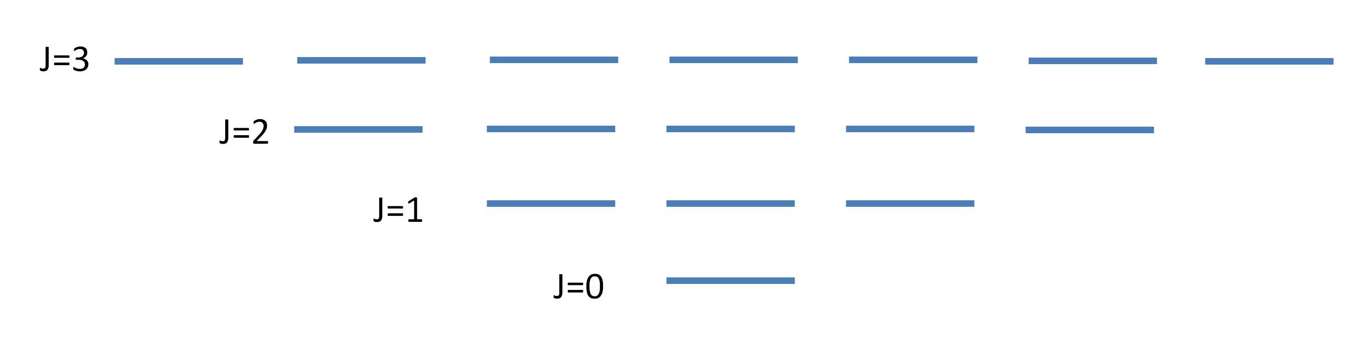
The solutions form a set of \(2J + 1\) eigenstates at each energy

\[E(J) = \dfrac{\hbar^2J(J+1)}{2I}.\]

A set of levels that are equal in energy is called a degenerate set as discussed within the context of 2D and 3D particle in boxes.

• \(J=0\): The lowest energy state has \(J = 0\) and \(m_J = 0\). This state has an energy \(E_0 = 0\). There is only one state with this energy, i.e. one set of quantum numbers, one wavefunction, and one set of properties for the molecule.
• \(J=1\): The next energy level is \(J = 1\) with energy \[E(J=1)=\dfrac {2\hbar ^2}{2I}.\] There are three states with this energy because \(m_J\) can equal +1, 0, or ‑1. These different states correspond to different orientations of the rotating molecule in space. States with the same energy are said to be degenerate. The degeneracy of an energy level is the number of states with that energy. The degeneracy of the \(J = 1\) energy level is 3 because there are three states with the energy \(\dfrac {2\hbar ^2}{2I}\).
• \(J=2\): The next energy level is for \(J = 2\). The energy is \[E(J=2)=\dfrac {6\hbar ^2}{2I},\] and there are five states with this energy corresponding to \(m_J = +2, \,+1,\, 0,\, ‑1,\, ‑2\). The energy level degeneracy is five. Note that the spacing between energy levels increases as J increases. Also note that the degeneracy increases. The degeneracy is always \(2J+1\) because \(m_J\) ranges from \(+J\) to \(‑J\) in integer steps, including 0.

Exercise

Calculate the possible angles a \(J = 1\) angular momentum vector can have with respect to the z-axis.

Exercise

What is the rotational energy and angular momentum of a molecule in the state with \(J = 0\)? Describe the rotation of a molecule in this state.

Uncertainty in Rotations (Vectoral Picture)

The classical definition of the orbital angular momentum vector of such a particle about the origin is \({\bf L} = {\bf x}\times{\bf p}\), giving (i.e., via the cross product):

\[ \hat{L}_x = y\, \hat{p}_z - z\, \hat{p}_y, \label{6.3.1a}\]

\[ \hat{L}_y = z\, \hat{p}_x - x\, \hat{p}_z \label{6.3.1b}\]

\[ \hat{L}_z = x\, \hat{p}_y - y \, \hat{p}_x \label{6.3.1c}\]

In Cartesian coordinates, the three components of orbital angular momentum can be written

\[\hat{L}_x = -{\rm i}\,\hbar\left(y\,\dfrac{\partial}{\partial z} - z\,\dfrac{\partial} {\partial y}\right) \label{6.3.2a}\]

\[ \hat{L}_y = -{\rm i}\,\hbar\left(z\,\dfrac{\partial}{\partial x} - x\,\dfrac{\partial} {\partial z}\right) \label{6.3.2b}\]

\[ \hat{L}_z = -{\rm i}\,\hbar\left(x\,\dfrac{\partial}{\partial y} - y\,\dfrac{\partial} {\partial x}\right) \label{6.3.2c}\]

using the Schrödinger representation. \(L_x\), \(L_y\), and \(L_z\) can, in principle, be measured. However, to determine if they can be measured simultaneously with infinite precision, these operators must commute.

Reminder: Heisenberg's Uncertainty Principle for linear momentum and position

Remember that the fundamental commutation relations satisfied by the position and linear momentum operators are:

\[[x_i, x_j] =0 \label{6.3.12}\]

\[[p_i, p_j] =0 \label{6.3.13}\]

\[[x_i, p_j] = i\,\hbar \,\delta_{ij} \label{6.3.14}\]

where \(i\) and \(j\) stand for either \(x\), \(y\), or \(z\).

Consider the commutator of the operators \(L_x\) and \(L_z\) :

\[ \begin{align*} [L_x, L_y] & = [(y\,p_z-z\,p_y), (z\,p_x-x \,p_z)] \\[4pt] &= y\,[p_z, z]\,p_x + x\,p_y\,[z, p_z] \label{6.3.15} \\[4pt] &= {\rm i}\,\hbar\,(-y \,p_x+ x\,p_y) = {\rm i}\,\hbar\, L_z \label{6.3.16} \end{align*}\]

This is one example of several cyclic permutations of the fundamental commutation relations satisfied by the components of an orbital angular momentum:

\[[\hat{L}_x, \hat{L}_y] = {\rm i}\,\hbar\, L_z \label{6.3.17a}\]

\[[ \hat{L}_y, \hat{L}_z] = {\rm i}\,\hbar\, L_x \label{6.3.17b}\]

\[[ \hat{L}_z, \hat{L}_x] = {\rm i}\,\hbar\, L_y \label{6.3.17c}\]

Therefore, two orthogonal components of angular momentum (for example \(L_x\) and \(L_y\)) are complementary and cannot be simultaneously known or measured, except in special cases such as \(\displaystyle L_{x}=L_{y}=L_{z}=0\), which means there is no rotation.

We can introduce a new operator \(\hat{L^2}\):

\[\hat{L^2} = L_x^{\,2}+L_y^{\,2}+L_z^{\,2} \label{6.3.5}\]

That is the magnitude of the Angular momentum squared.

It is possible to simultaneously measure or specify \(L^2\) (the eigen value, not the operator) and any single component of \(L\); for example, \(L^2\) and \(L_z\). This is often useful, and the values are characterized by (\(J\)) and (\(m_J\)). In this case, the quantum state of the system is a simultaneous eigenstate of the operators \(\hat{L^2}\) and \(\hat{L_z}\), but not of \(\hat{L_x}\) or \(\hat{L_y}\).

Illustration of the vector model of orbital angular momentum. (Public domain; Maschen).

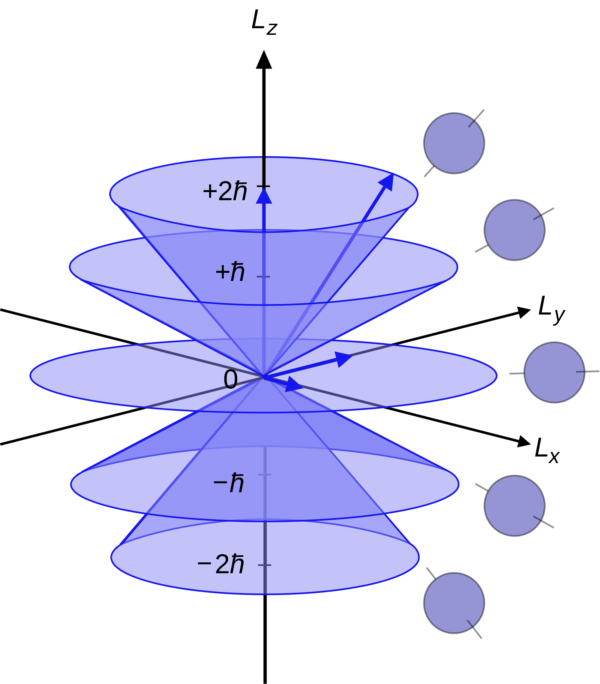
Since the angular momenta are quantum operators, they cannot be drawn as vectors like in classical mechanics. Nevertheless, it is common to depict them heuristically in this way. Depicted above is a set of states with quantum numbers \({\displaystyle J =2}\), and \({\displaystyle m_{J}=-2,-1,0,1,2}\) for the five cones from bottom to top.

Since \({\displaystyle |L|={\sqrt {L^{2}}}=\hbar {\sqrt {6}}}\), the vectors are all shown with length \({\displaystyle \hbar {\sqrt {6}}}\). The rings represent the fact that \({\displaystyle L_{z}}\) is known with certainty, but \({\displaystyle L_{x}}\) and \({\displaystyle L_{y}}\) are unknown; therefore every classical vector with the appropriate length and z-component is drawn, forming a cone.

The expected value of the angular momentum for a given ensemble of systems in the quantum state characterized by \({\displaystyle J}\) and \({\displaystyle m_{J }}\) could be somewhere on this cone while it cannot be defined for a single system (since the components of \({\displaystyle L}\) do not commute with each other).

Contributors and Attributions

• David M. Hanson, Erica Harvey, Robert Sweeney, Theresa Julia Zielinski ("Quantum States of Atoms and Molecules")