
12: Vibrational Spectroscopy of Diatomic Molecules
- Page ID
- 39041

\( \newcommand{\vecs}[1]{\overset { \scriptstyle \rightharpoonup} {\mathbf{#1}} } \)
\( \newcommand{\vecd}[1]{\overset{-\!-\!\rightharpoonup}{\vphantom{a}\smash {#1}}} \)
\( \newcommand{\dsum}{\displaystyle\sum\limits} \)
\( \newcommand{\dint}{\displaystyle\int\limits} \)
\( \newcommand{\dlim}{\displaystyle\lim\limits} \)
\( \newcommand{\id}{\mathrm{id}}\) \( \newcommand{\Span}{\mathrm{span}}\)
( \newcommand{\kernel}{\mathrm{null}\,}\) \( \newcommand{\range}{\mathrm{range}\,}\)
\( \newcommand{\RealPart}{\mathrm{Re}}\) \( \newcommand{\ImaginaryPart}{\mathrm{Im}}\)
\( \newcommand{\Argument}{\mathrm{Arg}}\) \( \newcommand{\norm}[1]{\| #1 \|}\)
\( \newcommand{\inner}[2]{\langle #1, #2 \rangle}\)
\( \newcommand{\Span}{\mathrm{span}}\)
\( \newcommand{\id}{\mathrm{id}}\)
\( \newcommand{\Span}{\mathrm{span}}\)
\( \newcommand{\kernel}{\mathrm{null}\,}\)
\( \newcommand{\range}{\mathrm{range}\,}\)
\( \newcommand{\RealPart}{\mathrm{Re}}\)
\( \newcommand{\ImaginaryPart}{\mathrm{Im}}\)
\( \newcommand{\Argument}{\mathrm{Arg}}\)
\( \newcommand{\norm}[1]{\| #1 \|}\)
\( \newcommand{\inner}[2]{\langle #1, #2 \rangle}\)
\( \newcommand{\Span}{\mathrm{span}}\) \( \newcommand{\AA}{\unicode[.8,0]{x212B}}\)
\( \newcommand{\vectorA}[1]{\vec{#1}} % arrow\)
\( \newcommand{\vectorAt}[1]{\vec{\text{#1}}} % arrow\)
\( \newcommand{\vectorB}[1]{\overset { \scriptstyle \rightharpoonup} {\mathbf{#1}} } \)
\( \newcommand{\vectorC}[1]{\textbf{#1}} \)
\( \newcommand{\vectorD}[1]{\overrightarrow{#1}} \)
\( \newcommand{\vectorDt}[1]{\overrightarrow{\text{#1}}} \)
\( \newcommand{\vectE}[1]{\overset{-\!-\!\rightharpoonup}{\vphantom{a}\smash{\mathbf {#1}}}} \)
\( \newcommand{\vecs}[1]{\overset { \scriptstyle \rightharpoonup} {\mathbf{#1}} } \)
\(\newcommand{\longvect}{\overrightarrow}\)
\( \newcommand{\vecd}[1]{\overset{-\!-\!\rightharpoonup}{\vphantom{a}\smash {#1}}} \)
\(\newcommand{\avec}{\mathbf a}\) \(\newcommand{\bvec}{\mathbf b}\) \(\newcommand{\cvec}{\mathbf c}\) \(\newcommand{\dvec}{\mathbf d}\) \(\newcommand{\dtil}{\widetilde{\mathbf d}}\) \(\newcommand{\evec}{\mathbf e}\) \(\newcommand{\fvec}{\mathbf f}\) \(\newcommand{\nvec}{\mathbf n}\) \(\newcommand{\pvec}{\mathbf p}\) \(\newcommand{\qvec}{\mathbf q}\) \(\newcommand{\svec}{\mathbf s}\) \(\newcommand{\tvec}{\mathbf t}\) \(\newcommand{\uvec}{\mathbf u}\) \(\newcommand{\vvec}{\mathbf v}\) \(\newcommand{\wvec}{\mathbf w}\) \(\newcommand{\xvec}{\mathbf x}\) \(\newcommand{\yvec}{\mathbf y}\) \(\newcommand{\zvec}{\mathbf z}\) \(\newcommand{\rvec}{\mathbf r}\) \(\newcommand{\mvec}{\mathbf m}\) \(\newcommand{\zerovec}{\mathbf 0}\) \(\newcommand{\onevec}{\mathbf 1}\) \(\newcommand{\real}{\mathbb R}\) \(\newcommand{\twovec}[2]{\left[\begin{array}{r}#1 \\ #2 \end{array}\right]}\) \(\newcommand{\ctwovec}[2]{\left[\begin{array}{c}#1 \\ #2 \end{array}\right]}\) \(\newcommand{\threevec}[3]{\left[\begin{array}{r}#1 \\ #2 \\ #3 \end{array}\right]}\) \(\newcommand{\cthreevec}[3]{\left[\begin{array}{c}#1 \\ #2 \\ #3 \end{array}\right]}\) \(\newcommand{\fourvec}[4]{\left[\begin{array}{r}#1 \\ #2 \\ #3 \\ #4 \end{array}\right]}\) \(\newcommand{\cfourvec}[4]{\left[\begin{array}{c}#1 \\ #2 \\ #3 \\ #4 \end{array}\right]}\) \(\newcommand{\fivevec}[5]{\left[\begin{array}{r}#1 \\ #2 \\ #3 \\ #4 \\ #5 \\ \end{array}\right]}\) \(\newcommand{\cfivevec}[5]{\left[\begin{array}{c}#1 \\ #2 \\ #3 \\ #4 \\ #5 \\ \end{array}\right]}\) \(\newcommand{\mattwo}[4]{\left[\begin{array}{rr}#1 \amp #2 \\ #3 \amp #4 \\ \end{array}\right]}\) \(\newcommand{\laspan}[1]{\text{Span}\{#1\}}\) \(\newcommand{\bcal}{\cal B}\) \(\newcommand{\ccal}{\cal C}\) \(\newcommand{\scal}{\cal S}\) \(\newcommand{\wcal}{\cal W}\) \(\newcommand{\ecal}{\cal E}\) \(\newcommand{\coords}[2]{\left\{#1\right\}_{#2}}\) \(\newcommand{\gray}[1]{\color{gray}{#1}}\) \(\newcommand{\lgray}[1]{\color{lightgray}{#1}}\) \(\newcommand{\rank}{\operatorname{rank}}\) \(\newcommand{\row}{\text{Row}}\) \(\newcommand{\col}{\text{Col}}\) \(\renewcommand{\row}{\text{Row}}\) \(\newcommand{\nul}{\text{Nul}}\) \(\newcommand{\var}{\text{Var}}\) \(\newcommand{\corr}{\text{corr}}\) \(\newcommand{\len}[1]{\left|#1\right|}\) \(\newcommand{\bbar}{\overline{\bvec}}\) \(\newcommand{\bhat}{\widehat{\bvec}}\) \(\newcommand{\bperp}{\bvec^\perp}\) \(\newcommand{\xhat}{\widehat{\xvec}}\) \(\newcommand{\vhat}{\widehat{\vvec}}\) \(\newcommand{\uhat}{\widehat{\uvec}}\) \(\newcommand{\what}{\widehat{\wvec}}\) \(\newcommand{\Sighat}{\widehat{\Sigma}}\) \(\newcommand{\lt}{<}\) \(\newcommand{\gt}{>}\) \(\newcommand{\amp}{&}\) \(\definecolor{fillinmathshade}{gray}{0.9}\)Last lecture continued the discussion of vibrations into the realm of quantum mechanics. We reviewed the classical picture of vibrations including the classical potential, bond length, and bond energy. We then introduced the quantum version using the harmonic oscillator as an approximation of the true potential. This involves constructing a Hamilonian with a parabolic potential. Solving the resulting (time-independent) Schrödinger equation to obtain the eigeinstates, energies, and quantum numbers (v) results is beyond this course, so they are given. Key aspect of these solutions are the fundamental frequency and zero-point energy.
Vibrations
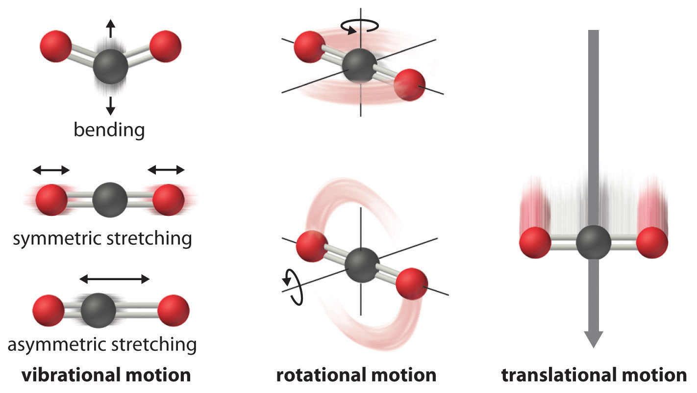
The motion of two particles in space can be separated into translational, vibrational, and rotational motions.
IR spectroscopy which has become so useful in identification, estimation, and structure determination of compounds draws its strength from being able to identify the various vibrational modes of a molecule. A complete description of these vibrational normal modes, their properties and their relationship with the molecular structure is the subject of this article.
Degree of freedom is the number of variables required to describe the motion of a particle completely. For an atom moving in 3-dimensional space, three coordinates are adequate so its degree of freedom is three. Its motion is purely translational. If we have a molecule made of N atoms (or ions), the degree of freedom becomes 3N, because each atom has 3 degrees of freedom. Furthermore, since these atoms are bonded together, all motions are not translational; some become rotational, some others vibration.
The degrees of vibrational modes for linear molecules can be calculated using the formula:
\[3N-5 \label{1}\]
The degrees of freedom for nonlinear molecules can be calculated using the formula:
\[3N-6 \label{2}\]
\(n\) is equal to the number of atoms within the molecule of interest. The following procedure should be followed when trying to calculate the number of vibrational modes:
- Determine if the molecule is linear or nonlinear (i.e. Draw out molecule using VSEPR). If linear, use Equation \ref{1}. If nonlinear, use Equation \ref{2}
- Calculate how many atoms are in your molecule. This is your \(N\) value.
- Plug in your \(N\) value and solve.
| Atoms (very symmetric) | Linear molecules (less symmetric) | Non-linear molecules (most unsymmetric) | |
|---|---|---|---|
| Translation (x, y, and z) | 3 | 3 | 3 |
| Rotation (x, y, and z) | 0 | 2 | 3 |
| Vibrations | 0 | 3N − 5 | 3N − 6 |
| Total (including Vibration) | 3 | 3N | 3N |
How many vibrational modes does water have?
- Answer
-
- The Symmetric Stretch (Example shown is an H2O molecule at 3685 cm-1)
- The Asymmetric Stretch (Example shown is an H2O molecule at 3506 cm-1)
- Bend (Example shown is an H2O molecule at 1885 cm-1)
A linear molecule will have another bend in a different plane that is degenerate or has the same energy. This accounts for the extra vibrational mode.
How many vibrational modes does carbon dioxide have?
- Answer
-
- Answer
-

It is important to note that there are many different kinds of bends, but due to the limits of a 2-dimensional surface it is not possible to show the other ones.
The frequencies of these vibrations depend on the inter-atomic binding energies which determines the force needed to stretch or compress a bond.
Properties of a Molecular Bond
- Breaking a bond always requires energy and hence making bonds always release energy.
- Bond length
- Bond energy (or enthalpy or strength)
The potential energy of a system of two atoms depends on the distance between them. At large distances the energy is zero, meaning “no interaction”. At distances of several atomic diameters attractive forces dominate, whereas at very close approaches the force is repulsive, causing the energy to rise. The attractive and repulsive effects are balanced at the minimum point in the curve.
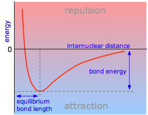
The internuclear distance at which the potential energy minimum occurs defines the bond length. This is more correctly known as the equilibrium bond length, because the two atoms will always vibrate about this distance.
Bond lengths depend mainly on the sizes of the atoms, and secondarily on the bond strengths, the stronger bonds tending to be shorter. Bonds involving hydrogen can be quite short; The shortest bond of all, H–H, is only 74 pm. Multiply-bonded atoms are closer together than singly-bonded ones; this is a major criterion for experimentally determining the multiplicity of a bond. This trend is clearly evident in the above plot which depicts the sequence of carbon-carbon single, double, and triple bonds.
In general, the stronger the bond, the smaller will be the bond length.
Reduced mass (Converting two atoms moving into one)
The internal motions of vibration and rotation for a two-particle system can be described by a single reduced particle with a reduced mass \(μ\) located at \(r\). In the below figure, the vector \(\vec{r}\) corresponds to the internuclear axis. The magnitude or length of \(r\) is the bond length, and the orientation of \(r\) in space gives the orientation of the internuclear axis in space. Changes in the orientation correspond to rotation of the molecule, and changes in the length correspond to vibration. The change in the bond length from the equilibrium bond length is the vibrational coordinate for a diatomic molecule.
The diagram shows the coordinate system for a reduced particle. \(R_1\) and \(R_2\) are vectors to \(m_1\) and \(m_2\). \(R\) is the resultant and points to the center of mass. (b) Shows the center of mass as the origin of the coordinate system, and (c) expressed as a reduced particle.
The Classical Harmonic Oscillator
Simple harmonic oscillators about a potential energy minimum can be thought of as a ball rolling frictionlessly in a dish (left) or a pendulum swinging frictionlessly back and forth. The restoring forces are precisely the same in either horizontal direction.

Simple image of a ball oscillating in a potential. from Wikipedia.
Recall that the Hamiltonian operator \(\hat{H}\) is the summation of the kinetic and potential energy in a system. There are several ways to approximate the potential function \(V\), but the two main means of approximation are done by using a Taylor series expansion, and the Morse Potential. The vibration of a diatomic is akin to an oscillating mass on a spring.
An undamped spring–mass system undergoes simple harmonic motion. from Wikipedia.
The classical forces in chemical bonds can be described to a good approximation as spring-like or Hooke's law type forces. This is true provided the energy is not too high. Of course, at very high energy, the bond reaches its dissociation limit, and the forces deviate considerably from Hooke's law. It is for this reason that it is useful to consider the quantum mechanics of a harmonic oscillator.
We will start in one dimension. Note that this is a gross simplification of a real chemical bond, which exists in three dimensions, but some important insights can be gained from the one-dimensional case. The Hooke's law force is
\[F(x)=-k(x-x_0)\]
where \(k\) is the spring constant. This force is derived from a potential energy
\[V(x)=\dfrac{1}{2}k(x-x_0)^2\]
Let us define the origin of coordinates such that \(x_0 =0\). Then the potential energy
\[ \color{red} V(x)=\dfrac{1}{2}kx^2\]
If a particle of mass \(m\) is subject to the Hooke's law force, then its classical energy is
\[\dfrac{p^2}{2m}+\dfrac{1}{2}kx^2 =E\]
Thus, we can set up the Schrödinger equation:
\[\left [ -\dfrac{\hbar^2}{2m}\dfrac{d^2}{dx^2}+\dfrac{1}{2}kx^2 \right ]\psi (x)=E\psi (x)\]
In this case, the Hamiltonian is
\[\hat{H}=-\dfrac{\hbar^2}{2m}\dfrac{d^2}{dx^2}+\dfrac{1}{2}kx^2\]
Since \(x\) now ranges over the entire real line \(x\in(-\infty ,\infty)\), the boundary conditions on \(\psi (x)\) are conditions at \(x=\pm \infty\). At \(x= \pm \infty\), the potential energy becomes infinite. Therefore, it must follow that as \(x \rightarrow \pm \infty\), \(\psi (x)\rightarrow 0\). Hence, we can state the boundary conditions as \(\psi (\pm \infty)=0\).
Solving this differential equation is not an easy task, so we will not attempt to do it. Here, we simply quote the allowed energies and some of the wave functions. The allowed energies are characterized by a single integer \(v\), which can be \(0,1,2,...\) and take the form
where \(\nu\) is the frequency of the oscillation (of a single mass on a spring):
\(\nu_1\) is the fundamental frequency of the mechanical oscillator which depends on the force constant of the spring and a single mass of the attached (single) body and independent of energy imparted on the system. when there are two masses involved in the system (e.g., a vibrating diatomic), then the mass used in Equation \(\ref{BigEq}\) becomes is a reduced mass:
\[ \color{red} \mu = \dfrac{m_1 m_2}{m_1+m_2} \label{14}\]
The fundamental vibrational frequency is then rewritten as
\[\nu = \dfrac{1}{2\pi} \sqrt{\dfrac{k}{\mu}} \label{15}\]
Do not confuse \(v\) the quantum number for harmonic oscillator with \(\nu\) the fundamental frequency of the vibration
The natural frequency \(\nu\) can be converted to angular frequency \(\omega\) via
\[\omega = 2\pi \nu\]
Then the energies in Equation \(\ref{BigEq}\) can be rewritten in terms of the fundamental angular frequency as
Now the eigenstates
Now we can define the parameter (for convenience)
the first few wave functions are
\[\begin{align*}\psi_0 (x) &= \left ( \dfrac{\alpha}{\pi} \right )^{1/4}e^{-\alpha x^2 /2}\\ \psi_1(x) &= \left ( \dfrac{4\alpha ^3}{\pi} \right )^{1/4}xe^{-\alpha x^2 /2}\\ \psi_2 (x) &= \left ( \dfrac{\alpha}{4\pi} \right )^{1/4}(2\alpha x^2 -1)e^{-\alpha x^2/2}\\ \psi_3 (x) &= \left ( \dfrac{\alpha ^3}{9\pi} \right )^{1/4}(2\alpha x^3 -3x)e^{- \alpha x^2 /2}\end{align*}\]
You should verify that these are in fact solutions of the Schrödinger equation by substituting them back into the equation with their corresponding energies. The figure below shows these wave functions
The harmonic oscillator wavefunctions describing the four lowest energy states.
The figure below shows these wave functions and the corresponding probability densities: \(p_n (x)=\psi_{n}^{2}(x)\):
The probability densities for the four lowest energy states of the harmonic oscillator.
Note that in contrast to a particle in an infinite high box, \(x\epsilon (-\infty ,\infty)\), so the normalization condition for each eignestate is
\[\int_{-\infty}^{\infty}\psi_{n}^{2}(x)dx=1\]
Despite this, because the potential energy rises very steeply, the wave functions decay very rapidly as \(|x|\) increases from 0 unless \(n\) is very large. This is discussed as tunneling elsewhere. (See https://phet.colorado.edu/en/simulation/bound-states)

Another way to show solutions to harmonic oscillators. (left) Wavefunction representations for the first eight bound eigenstates, n = 0 to 7. The horizontal axis shows the position x. Note: The graphs are not normalized, and the signs of some of the functions differ from those given in the text. (right) Corresponding probability densities.Images used with permission (CC BY-SA 3.0; AllenMcC.).
Contributors and Attributions
David M. Hanson, Erica Harvey, Robert Sweeney, Theresa Julia Zielinski ("Quantum States of Atoms and Molecules")
William Reusch, Professor Emeritus (Michigan State U.), Virtual Textbook of Organic Chemistry