Homework 9 Key

Q1

Find the spectroscopic terms originating from the following configurations (two electrons in two non-equivalent orbitals in the same atom):

The spectroscopic terms are ^{2S + 1}L_J where S = |m_s1 + m_s2|, |m_s1 + m_s2 - 1|, ...., |m_s1 - m_s2|, L = |l₁ + l₂|, |l₁ + l₂ - 1|, ...., |l₁ - l₂|, and J = |L + S|, |L + S - 1|, ...., |L - S| and since the two electrons in each example are in different orbitals, i.e. 2p3p instead of 2p2p, we do not have to worry about the Pauli exclusion principle rendering certain terms impossible.

a) 1s2s = ³S₁ ¹S₀

b) 1s3s = ³S₁ ¹S₀

c) 2p3p = ³D₃ ³D₂ ³D₁ ¹D₂ ³P₂ ³P₁ ³P₀ ¹P₁ ³S₁ ¹S₀

d) 2s3d = ³D₃ ³D₂ ³D₁ ¹D₂

Q2

This is a complex question for several reasons. Previously, we considered excited state as only different electron configurations. However, now we can differentiate levels based on term symbols (microstates). So different microstates will have the same electron configuration. The second aspect is how to identify which state is lower or higher in energy. While technically, Hund's rule applies to only ground-state, the gist of the rules can be be use for higher state (just do not rely exclusively on them).

The first step in identifying microstates and assigning term symbols is to establsih electron configurations

First excited states:

H: This is a one electron system. The first excited state based off of electron configuration will have a 2s configuration. This is a \(^2S_{1/2}\) state.

He: This is a two electron system. The first excited state based off of electron configuration will have a 1s¹2s¹ configuration. There are two microstates for this configuration: \(^3S_{1}\) (spin aligned) and \(^1S_{0}\). Hund's first rule predicts the triplet state is the lowest of this configuration (it is too)

Li: This is a three electron system. The first excited state based off of electron configuration will have a 1s²2s⁰2p¹ configuration. There are two microstates for this configuration: \(^2P_{1/2}\) and \(^2P_{3/2}\). Since the p-orbitals are less than half-full, the term with the lowest J will be lower in energy (Hund's third rule); therefore, the lowest excited state will be \(^2P_{1/2}\).

Be: This is a four electron system. The first excited state based off of electron configuration will have a 1s²2s¹2p¹ configuration. There are two microstates for this configuration: \(^1P_{1}\) and \(^3P_1\). The triplet is preferred via Hund's first rule

B: This is a five electron system. The first excited state based off of electron configuration will have a 1s²2s²3s¹ configuration, This would have a \(^2S_{1/2}\) state. However, the ground-state configuration 1s²2s²2p¹ has multiple states in it, so one of those is really the first excited-state.

For C, N and O, the electron configuration is the same as for the ground state, but the occupation of degenerate p-orbitals is not optimal.

C: 2s²2p² which is a ¹D

N: 2s²2p³ which is a ²D

O: 2s²2p⁴ which is a ¹D

F: 2s²2p⁵ which is a ²P

Ne: 2s²2p⁵3s¹ which is a ³P

Q3

Find the spectroscopic term originating from the ground states configuration of the sodium atom and the boron atom.

Al: [Ne]3s²3p¹ so with one 2p electron not in a filled shell our terms are ²P_3/2 and ²P_1/2

Na: [Ne]3s¹ so with one 3s electron not in a filled shell our term is ²S_1/2

Q4

2p: ²P_3/2 and ²P_1/2

3d: ²D_5/2 ²D_3/2

Q5

a) Be ----> Be⁺ + e^-

b) Be: 1s²2s², so the term symbol is ¹S₀, because it is a closed shell system;

Be+: 1s²2s¹, so L=0, S=1/2, term symbol is: ²S_1/2

c) Electronic energy for Be is: -9143.9 kcal/mol

Electronic energy for Be+ is: -8958.45 kcal/mol

So the ionization energy is: -8958.45 - (-9143.9) = 185.45 kcal/mol.

d) For neutral atom Be, the energy of the highest occupied orbital is -193.8 kcal/mol (the second energy value for "Orbital Energies" on the output page of ChemCompute). So, according to Koopman's theorem, the first ionization energy is -(-193.8)=193.8 kcal/mol.

e) The difference between Koopman theorem value and normal calculation value is: 193.8-185.45=8.35 kcal/mol. It is 8.35/185.45=4.5% of the normal calculation value. Its accurary is due to the assumption of frozen orbitals, i.e., when you remove an electron from the highest occupied orbital, the rest of the orbitals do not change. And this is a pretty good assumption for beryllium. However, if you do not assume frozen orbitals, then, when you remove an electron, the rest of the orbitals are going to change and you will not be able to assume E_Ionization=E_N-1-E_N=-ε_k.

To help you understand better, I will explain the terms in the equation above:

E_Ionization=E_N-1-E_N, this part is the normal way how you calculate ionization energy, without considering Koopman's theorem.

E_Ionization=-ε_k is the energy that you would get if you use Koopman's theorem.

So taken together, according to Koopman's theorem, ideally if the frozen orbitals assumption is true, you should get E_Ionization=E_N-1-E_N=-ε_k. However, if the frozen orbitals assumption is not describing the real situation that is going in the molecule very well, then you will find that E_N-1-E_N and -ε_k have different values_. But Normally, these two values are very close to each other, becasue the frozen orbitals assumption can usually describe the molecule pretty accurately.

Q6

For (a) and (b), just expand the original determinant and the determinants with interchanged rows or columns, and compare the results. You will find that interchanging two rows or columns will lead to the change of sign.

(c) Assuming \(\psi_A =\psi_B\), then we get two identical rows in the determinant. According to matrix algebra, the determinant with two identical rows equals to zero. So, we get an invalid wavefunction, because a valid wavefunction cannot be zero all the time.

Q7

\[\psi_1 = \frac{1}{2}[\phi_1(1)\phi_2(2) + \phi_1(2)\phi_2(1)][\alpha(1)\beta(2)-\beta(1)\alpha(2)]\]

\[=\dfrac{1}{2}[ \phi_1(1)\phi_2(2)\alpha(1)\beta(2)-\phi_1(1)\phi_2(2)\beta(1)\alpha(2)+\phi_1(2)\phi_2(1)\alpha(1)\beta(2) -\phi_1(2)\phi_2(1)\beta(1)\alpha(2) \]

\[=\dfrac{1}{2}[ \phi_1(1)\alpha(1)\phi_2(2)\beta(2)-\phi_1(2)\alpha(2)\phi_2(1)\beta(1) ]-\dfrac{1}{2}[ \phi_1(1)\beta(1)\phi_2(2)\alpha(2)-\phi_1(2)\beta(2)\phi_2(1)\alpha(1) ] \]

\[ = \dfrac{1}{2}\begin{vmatrix} \phi_1(1)\alpha(1) & \phi_2(1)\beta(1) \\ \phi_1(2)\alpha(2) & \phi_2(2)\beta(2) \end{vmatrix}-\dfrac{1}{2} \begin{vmatrix} \phi_1(1)\beta(1) & \phi_2(1)\alpha(1) \\ \phi_1(2)\beta(2) & \phi_2(2)\alpha(2) \end{vmatrix}\]

======================

\[\psi_2 = \frac{1}{\sqrt{2}}[\phi_1(1)\phi_2(2) - \phi_1(2)\phi_2(1)][\alpha(1)\alpha(2)] \]

\[=\frac{1}{\sqrt{2}}[\phi_1(1)\phi_2(2)\alpha(1)\alpha(2)-\phi_1(2)\phi_2(1)\alpha(1)\alpha(2)] \]

\[=\frac{1}{\sqrt{2}}[\phi_1(1)\alpha(1)\phi_2(2)\alpha(2)-\phi_1(2)\alpha(2)\phi_2(1)\alpha(1)] \]

\[=\frac{1}{\sqrt{2}} \begin{vmatrix} \phi_1(1)\alpha(1) & \phi_2(1)\alpha(1) \\ \phi_1(2)\alpha(2) & \phi_2(2)\alpha(2) \end{vmatrix} \]

=======================

\[\psi_3 = \frac{1}{\sqrt{2}}[\phi_1(1)\phi_2(2) - \phi_1(2)\phi_2(1)][\beta(1)\beta(2)]\]

\[=\frac{1}{\sqrt{2}}[\phi_1(1)\phi_2(2)\beta(1)\beta(2)-\phi_1(2)\phi_2(1)\beta(1)\beta(2)] \]

\[=\frac{1}{\sqrt{2}}[\phi_1(1)\beta(1)\phi_2(2)\beta(2)-\phi_1(2)\beta(2)\phi_2(1)\beta(1)] \]

\[=\frac{1}{\sqrt{2}} \begin{vmatrix} \phi_1(1)\beta(1) & \phi_2(1)\beta(1) \\ \phi_1(2)\beta(2) & \phi_2(2)\beta(2) \end{vmatrix} \]

========================

\[\psi_4 = \frac{1}{2}[\phi_1(1)\phi_2(2) - \phi_1(2)\phi_2(1)][\alpha(1)\beta(2)+\beta(1)\alpha(2)] \]

\[=\dfrac{1}{2}[ \phi_1(1)\phi_2(2)\alpha(1)\beta(2)+\phi_1(1)\phi_2(2)\beta(1)\alpha(2)-\phi_1(2)\phi_2(1)\alpha(1)\beta(2) -\phi_1(2)\phi_2(1)\beta(1)\alpha(2) \]

\[=\dfrac{1}{2}[ \phi_1(1)\alpha(1)\phi_2(2)\beta(2)-\phi_1(2)\alpha(2)\phi_2(1)\beta(1) ]+\dfrac{1}{2}[ \phi_1(1)\beta(1)\phi_2(2)\alpha(2)-\phi_1(2)\beta(2)\phi_2(1)\alpha(1) ] \]

\[ = \dfrac{1}{2}\begin{vmatrix} \phi_1(1)\alpha(1) & \phi_2(1)\beta(1) \\ \phi_1(2)\alpha(2) & \phi_2(2)\beta(2) \end{vmatrix}+\dfrac{1}{2} \begin{vmatrix} \phi_1(1)\beta(1) & \phi_2(1)\alpha(1) \\ \phi_1(2)\beta(2) & \phi_2(2)\alpha(2) \end{vmatrix}\]

Q8

\[\hat{H}_{H_2^+}(1) = \dfrac{-\hbar^2}{2m_{e1}}\nabla_{e1}^2 + \dfrac{e^2}{4\pi \epsilon_0 R} - \dfrac{e^2}{4\pi \epsilon_0} \left(\frac{1}{r_{1A}} + \dfrac{1}{r_{1B}} \right) \]

In the \(H_2^+\) hamiltonian the first term is the kinetic energy term for the electron, the second term is the coulomb repulsion between the nuclei, and the last terms contain the electron nuclei attraction terms.

\[\hat{H}_{H_2}(1,2) = \dfrac{-\hbar^2}{2m_{e1}}\nabla_{e1}^2 + \dfrac{-\hbar^2}{2m_{e2}}\nabla_{e2}^2 + \dfrac{e^2}{4\pi \epsilon_0 R} - \dfrac{e^2}{4\pi \epsilon_0} \left(\dfrac{1}{r_{1A}} + \dfrac{1}{r_{1B}} + \dfrac{1}{r_{2A}} + \dfrac{1}{r_{2B}}\right) + \dfrac{e^2}{4\pi \epsilon_0 r_{12}}\]

In the \(H_2\) Hamiltonian the first two terms are the kinetic terms for each electron, the third term is coulomb repulsion between nuclei A and B which under the Born-Oppenhiemer approximation is static, and the last terms contain the electron nuclei attraction and the electron and electron repulsion term.

The difference between the two Hamiltonians is that with the loss of the second electron you lose the kinetic and potential terms related to that electron as well as the electron-electron repulsion term.

Q9

The first thing to notice is that |c₁|² = |c₂|² since the electron should have no preference on which proton it is near, so their probabilities should be the same.

\[\langle \psi_{\pm} | \psi_{\pm} \rangle = |c_{\pm}|^2 \left(\int \phi_A^2 d\tau + \int \phi_B^2 d\tau \pm \int \phi_B \phi_A d\tau \pm \int \phi_A \phi_B d\tau \right) = 1\]

and

\[\int \phi_A^2 d\tau = \int \phi_B^2 d\tau = 1\]

since they are normalized atomic wavefunctions.

\[\langle \psi_{\pm} | \psi_{\pm} \rangle = |c_{\pm}|^2 (1 + 1 \pm (S + S^*)) = 1\]

Since both wavefunctions are real \(S = S^*\)

\[\langle \psi_{\pm} | \psi_{\pm} \rangle = |c_{\pm}|^2 (1 + 1 \pm 2S) = 1\]

\[|c_{\pm}| = (2 \pm 2S)^{-1/2}\]

Q10

Based on the electron density (Figure 9.3.1b) the ψ− orbital is higher in energy since it has more probability density on the outside of the nuclei while ψ+ has more density in the middle of the nuclei. When the electron is not in the middle of the nuclei there is no shielding between the two protons which repel each other creating a higher energy situation. ψ− is the orbital with a node in the middle of the two nuclei which make sense since it is the higher energy orbital.

Q11

These should look like the curves in Lecture 26 for the expressions for the integrals as a function of internuclear distance.

Q12

The overlap integral between an \(H_{2s}\) orbital and a \(H_{2s}\) orbital on nuclei separated by a distance \(R\) is:

\[S(2s,2s)=\left\{1 + \dfrac{R}{2a_0} + \dfrac{1}{12}\left(\dfrac{R}{a_0}\right)^2 + \dfrac{1}{240}\left(\dfrac{R}{a_0}\right)^4\right\} e^{-R/2a}\]

Created by Ghunbong Cheung in Adobe Flash CS6

To find where the overlap is at its maximum, we set

\[\dfrac{dS}{dR} = 0\]

\[-\dfrac{Re^{-R/{2a_0}}(40a_0^3+20a_0^2R-8a_0R^2+R^3)}{480a_0^5} = 0\]

There are four roots for \(R\) since it is a quartic polynomial, but only one logical solution:

\[R = 0\]

Created by Ghunbong Cheung in MATLAB

This solution makes sense because these two orbitals are identical, so the maximum overlap should logical occur when the orbitals are exactly on top of each other.

Q13

The bond order for \(H_2^+\) is \(1/2\) as there is a single bonding electron. For \(H_2\) the bond order is 1. So with double the bond order you might expect \(H_2\) to have double the dissociation energy. However \( 436 < 2D_{H_2^+} \) so in \(H_2\) there is an additional term in the Hamiltonian not present in \(H_2^+\) which is reducing the well depth and the dissociation energy. The nuclear repulsion is already accounted for in \(H_2^+\) but the electron repulsion is not. This additional repulsion factor is responsible for the change in dissociation energy between \(H_2^+\) and \(H_2\).

Another way to look at this that the one electron shields the nuclear charge of the other.

Q14

Probability of finding an electron is given by \(P = \Big|\psi^2\Big|d\tau\).

We know that \(R = 106\;\text{pm}\) for H₂⁺.

For the bonding LCAO-MO,

\[\psi_+^2=C_+^2(1s_A+1s_B)^2\]

\[\psi_+^2=C_+^2\dfrac{1}{\pi a_0^3}\Big(e^{-r_A/a_0}+e^{-r_B/a_0}\Big)^2\]

\[C_+^2\dfrac{1}{\pi a_0^3} = (0.561)^2\times\left(\dfrac{1}{\pi\times(52.9\;\text{pm})^3}\right)=6.7672\times10^{-7}\;\text{pm}^{-3}\]

(a) at nucleus A, \(r_A=0\) and \(r_B = R\):

\[\psi_+^2=8.72\times10^{-7}\;\text{pm}^{-3}\]

\[P = (8.72\times10^{-7}\;\text{pm}^{-3})\times(2.00\;\text{pm}^3) = 1.72\times10^{-6}\]

(b) at nucleus B:

\[P = 1.72\times10^{-6}\]

due to symmetry

(c) halfway between A and B, \(r_A=\dfrac{1}{2}R\) and \(r_B=\dfrac{1}{2}R\)

\[\psi_+^2=3.7\times10^{-7}\;\text{pm}^{-3}\]

\[P = \Big(3.7\times10^{-7}\;\text{pm}^{-3}\Big)\times(2.00\;\text{pm}^3) = 7.4\times10^{-7}\]

(d) at a point 40 pm along the bond from A and 15 pm perpendicularly, \(r_A=42.7\;\text{pm}\) and \(r_B=67.7\;\text{pm}\), these values are found using Pythagorean Theorem.

\[\psi_+^2=(e^{-42.7/52.9}+e^{-67.7/52.9})^2\times(6.7672\times10^{-7}\;\text{pm}^{-3})=3.55\times10^{-7}\;\text{pm}^{-3}\]

\[P = 3.55\times10^{-7}\;\text{pm}^{-3}\times(2.00\;\text{pm}^3)=7.09\times10^{-7}\]

For the antibonding LCAO-MO

\[\psi_-^2=C_-^2(1s_A-1s_B)^2\]

\[\psi_-^2=C_-^2\dfrac{1}{\pi a_0^3}\Big(e^{-r_A/a_0}-e^{-r_B/a_0}\Big)^2\]

\[C_-^2\dfrac{1}{\pi a_0^3} = (1.10)^2\times\Big(\dfrac{1}{\pi\times(52.9\;\text{pm})^3}\Big)=2.6018\times10^{-7}\;\text{pm}^{-3}\]

(a) at nucleus A, \(r_A=0\) and \(r_B = R\):

\[\psi_-^2=19.6\times10^{-7}\;\text{pm}^{-3}\]

\[P = (19.6\times10^{-7}\;\text{pm}^{-3})\times(2.00\;\text{pm}^3) = 3.92\times10^{-6}\]

(b) at nucleus B:

\[P = 3.92\times10^{-6}\]

due to symmetry

(c) halfway between A and B, \(r_A=\dfrac{1}{2}R\) and \(r_B=\dfrac{1}{2}R\)

\[\psi_-^2=0\]

\[P = 0\]

(d) at a point 40 pm along the bond from A and 15 pm perpendicularly, \(r_A=42.7\;\text{pm}\) and \(r_B=67.7\;\text{pm}\), these values are found using Pythagorean Theorem.

\[\psi_-^2=(e^{-42.7/52.9}-e^{-67.7/52.9})^2\times(2.6018\times10^{-7}\;\text{pm}^{-3})=7.20\times10^{-8}\;\text{pm}^{-3}\]

\[P = 7.20\times10^{-8}\;\text{pm}^{-3}\times(2.00\;\text{pm}^3)=1.44\times10^{-7}\]

Q15

Species	Bond Order	Spin Multiplicity	Paramagnetic
B2	1	1	no
O2	2	3	yes
N2	3	1	no
N2^+	2.5	2	yes (weakly)
H2^+	0.5	2	yes (weakly)
\( (\sigma_{1s})^2 (\sigma^*_{1s})^2(\sigma_{2s})^2 (\sigma^*_{2s})^2(\pi_{2p})^2 \)	1	1	no
\( (\sigma_{1s})^2 (\sigma^*_{1s})^2(\sigma_{2s})^1 (\sigma^*_{2s})^1 \)	0	3 (assuming Hund's rule applies for this excited state)	yes (if the molecule exists)
\( (\sigma_{1s})^2 (\sigma^*_{1s})^2(\sigma_{2s})^2 (\sigma^*_{2s})^2 (\sigma_{2p_z})^2 (\pi_{2p})^4(\pi^*_{2p})^2 \) (This is isoelectronic with \(O_2\))	2	3	yes

Q16

We have to use the bond order formula for each of the situations.

\[\text{Bond order} = \dfrac{(\text{number of bonding electrons})- (\text{number of anti-bonding electrons})}{2} \]

For O₂: We have 12 valence electrons. Therefore

\[\text{Bond order} = \dfrac{10 - 6}{2} = 2\]

For O₂⁺: We have 11 valence electrons. Therefore

\[\text{Bond order} = \dfrac{10 - 5}{2} = \dfrac{5}{2}\]

For O₂^2-: We have 14 valence electrons. Therefore

\[\text{Bond order}= \dfrac{10 - 8}{2} = 1 \]

From the bond orders, we can see that O₂^2- is the least stable. A similar problems is also outline here in Lecture 27: Molecular Oxygen is Paramagnetic. If you desire a similar exercises to test your skills, substitute \(N\) for \(O\) in the problem and see how things change.

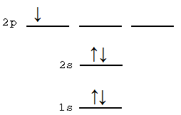
Q17

This is a five electron wavefunctions that may be assigned to an atom, not a molecule. This is because the orbital components of the determinant are orbitals are atomic, not molecular. For example,, this determinate wavefunction may be the \(B\) atom (although it could be an ion too) and corresponds to the following electron configuration: