Homework 6B: ab initio Calculations
- Page ID
- 143076
\( \newcommand{\vecs}[1]{\overset { \scriptstyle \rightharpoonup} {\mathbf{#1}} } \)
\( \newcommand{\vecd}[1]{\overset{-\!-\!\rightharpoonup}{\vphantom{a}\smash {#1}}} \)
\( \newcommand{\id}{\mathrm{id}}\) \( \newcommand{\Span}{\mathrm{span}}\)
( \newcommand{\kernel}{\mathrm{null}\,}\) \( \newcommand{\range}{\mathrm{range}\,}\)
\( \newcommand{\RealPart}{\mathrm{Re}}\) \( \newcommand{\ImaginaryPart}{\mathrm{Im}}\)
\( \newcommand{\Argument}{\mathrm{Arg}}\) \( \newcommand{\norm}[1]{\| #1 \|}\)
\( \newcommand{\inner}[2]{\langle #1, #2 \rangle}\)
\( \newcommand{\Span}{\mathrm{span}}\)
\( \newcommand{\id}{\mathrm{id}}\)
\( \newcommand{\Span}{\mathrm{span}}\)
\( \newcommand{\kernel}{\mathrm{null}\,}\)
\( \newcommand{\range}{\mathrm{range}\,}\)
\( \newcommand{\RealPart}{\mathrm{Re}}\)
\( \newcommand{\ImaginaryPart}{\mathrm{Im}}\)
\( \newcommand{\Argument}{\mathrm{Arg}}\)
\( \newcommand{\norm}[1]{\| #1 \|}\)
\( \newcommand{\inner}[2]{\langle #1, #2 \rangle}\)
\( \newcommand{\Span}{\mathrm{span}}\) \( \newcommand{\AA}{\unicode[.8,0]{x212B}}\)
\( \newcommand{\vectorA}[1]{\vec{#1}} % arrow\)
\( \newcommand{\vectorAt}[1]{\vec{\text{#1}}} % arrow\)
\( \newcommand{\vectorB}[1]{\overset { \scriptstyle \rightharpoonup} {\mathbf{#1}} } \)
\( \newcommand{\vectorC}[1]{\textbf{#1}} \)
\( \newcommand{\vectorD}[1]{\overrightarrow{#1}} \)
\( \newcommand{\vectorDt}[1]{\overrightarrow{\text{#1}}} \)
\( \newcommand{\vectE}[1]{\overset{-\!-\!\rightharpoonup}{\vphantom{a}\smash{\mathbf {#1}}}} \)
\( \newcommand{\vecs}[1]{\overset { \scriptstyle \rightharpoonup} {\mathbf{#1}} } \)
\( \newcommand{\vecd}[1]{\overset{-\!-\!\rightharpoonup}{\vphantom{a}\smash {#1}}} \)
\(\newcommand{\avec}{\mathbf a}\) \(\newcommand{\bvec}{\mathbf b}\) \(\newcommand{\cvec}{\mathbf c}\) \(\newcommand{\dvec}{\mathbf d}\) \(\newcommand{\dtil}{\widetilde{\mathbf d}}\) \(\newcommand{\evec}{\mathbf e}\) \(\newcommand{\fvec}{\mathbf f}\) \(\newcommand{\nvec}{\mathbf n}\) \(\newcommand{\pvec}{\mathbf p}\) \(\newcommand{\qvec}{\mathbf q}\) \(\newcommand{\svec}{\mathbf s}\) \(\newcommand{\tvec}{\mathbf t}\) \(\newcommand{\uvec}{\mathbf u}\) \(\newcommand{\vvec}{\mathbf v}\) \(\newcommand{\wvec}{\mathbf w}\) \(\newcommand{\xvec}{\mathbf x}\) \(\newcommand{\yvec}{\mathbf y}\) \(\newcommand{\zvec}{\mathbf z}\) \(\newcommand{\rvec}{\mathbf r}\) \(\newcommand{\mvec}{\mathbf m}\) \(\newcommand{\zerovec}{\mathbf 0}\) \(\newcommand{\onevec}{\mathbf 1}\) \(\newcommand{\real}{\mathbb R}\) \(\newcommand{\twovec}[2]{\left[\begin{array}{r}#1 \\ #2 \end{array}\right]}\) \(\newcommand{\ctwovec}[2]{\left[\begin{array}{c}#1 \\ #2 \end{array}\right]}\) \(\newcommand{\threevec}[3]{\left[\begin{array}{r}#1 \\ #2 \\ #3 \end{array}\right]}\) \(\newcommand{\cthreevec}[3]{\left[\begin{array}{c}#1 \\ #2 \\ #3 \end{array}\right]}\) \(\newcommand{\fourvec}[4]{\left[\begin{array}{r}#1 \\ #2 \\ #3 \\ #4 \end{array}\right]}\) \(\newcommand{\cfourvec}[4]{\left[\begin{array}{c}#1 \\ #2 \\ #3 \\ #4 \end{array}\right]}\) \(\newcommand{\fivevec}[5]{\left[\begin{array}{r}#1 \\ #2 \\ #3 \\ #4 \\ #5 \\ \end{array}\right]}\) \(\newcommand{\cfivevec}[5]{\left[\begin{array}{c}#1 \\ #2 \\ #3 \\ #4 \\ #5 \\ \end{array}\right]}\) \(\newcommand{\mattwo}[4]{\left[\begin{array}{rr}#1 \amp #2 \\ #3 \amp #4 \\ \end{array}\right]}\) \(\newcommand{\laspan}[1]{\text{Span}\{#1\}}\) \(\newcommand{\bcal}{\cal B}\) \(\newcommand{\ccal}{\cal C}\) \(\newcommand{\scal}{\cal S}\) \(\newcommand{\wcal}{\cal W}\) \(\newcommand{\ecal}{\cal E}\) \(\newcommand{\coords}[2]{\left\{#1\right\}_{#2}}\) \(\newcommand{\gray}[1]{\color{gray}{#1}}\) \(\newcommand{\lgray}[1]{\color{lightgray}{#1}}\) \(\newcommand{\rank}{\operatorname{rank}}\) \(\newcommand{\row}{\text{Row}}\) \(\newcommand{\col}{\text{Col}}\) \(\renewcommand{\row}{\text{Row}}\) \(\newcommand{\nul}{\text{Nul}}\) \(\newcommand{\var}{\text{Var}}\) \(\newcommand{\corr}{\text{corr}}\) \(\newcommand{\len}[1]{\left|#1\right|}\) \(\newcommand{\bbar}{\overline{\bvec}}\) \(\newcommand{\bhat}{\widehat{\bvec}}\) \(\newcommand{\bperp}{\bvec^\perp}\) \(\newcommand{\xhat}{\widehat{\xvec}}\) \(\newcommand{\vhat}{\widehat{\vvec}}\) \(\newcommand{\uhat}{\widehat{\uvec}}\) \(\newcommand{\what}{\widehat{\wvec}}\) \(\newcommand{\Sighat}{\widehat{\Sigma}}\) \(\newcommand{\lt}{<}\) \(\newcommand{\gt}{>}\) \(\newcommand{\amp}{&}\) \(\definecolor{fillinmathshade}{gray}{0.9}\)Name: ______________________________
Section: _____________________________
Student ID#:__________________________
adapted from Professor Delmar Larsen
This homework will introduce Quantum Mechanical Calculations. We will use the web based ab initio site by Perri at Sonoma State U. The following paper provides the background on this open source project (http://pubs.acs.org/doi/pdf/10.1021/ed5004228). Follow the directions on this assignment/tutorial. We will use this package multiple times in this class so make sure you can complete the online tutorial if you are confused.
To start the calculations
- click here: https://chemcompute.org
- Create an account using login/register.
- Click on GAMESS at the top or in the center of the home menu.
- Instructions are available below.
Method 1: The "Hard" Way
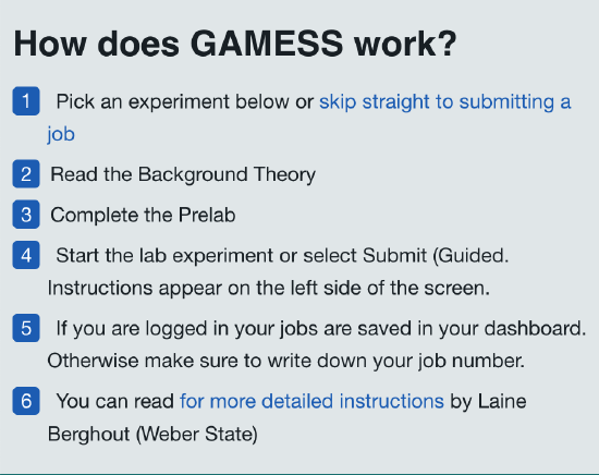
We're going to optimize the hydrogen atom. First, clicke the button "skip straight to submitting a job".
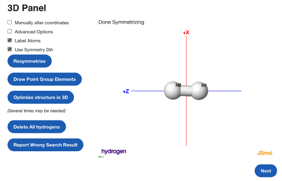
Next, search for a molecule "Hydrogen". Hopefully it looks like this! Click on the Next button.
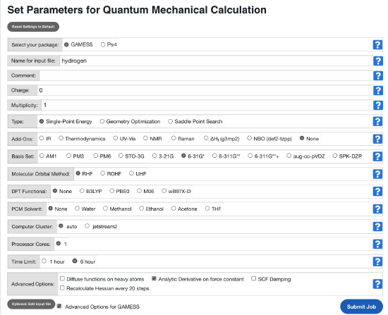
Feel free to add a comment. Otherwise, change the calculations as such:
Type: Single-point energy
Add-ons: None
Basis Set: 6-41G*
Molecular Orbital Method: RHF (Restricted Hartree-Fock Method)
No DFT Functional.
PCM Solvent: None
You can change your coordinates by clicking the grey button Edit input file. The input file will show up in a window below. Edit the values of the bond distances such as:
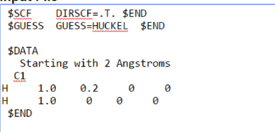
That's a 0.2 angstrom bond distance.
Submit your job.
The Easy Way
Alternatively, this calculation has been done many times. Type in 02588 in the "Read Geometry From a Previous Job" and press input. It pulls in all details from a previous calculation.

Type a name for your file, e.g. "H2_yourname" in step 4 "Name for input file"
Check "Single-Point Energy" next to "Type of Calculation" This will instruct GAMESS not to change your coordinates.
Click "Create input file" (step 5)
Click "Submit Job" (step 6). This may take a minute or two.
The difference between single-point calculations and geometry optimization is that that the former calculates the electron structure for one specific and given geometry; the later will do it at a series of geometries while decreasing the total energy of the system.
The Output
The output will look like this
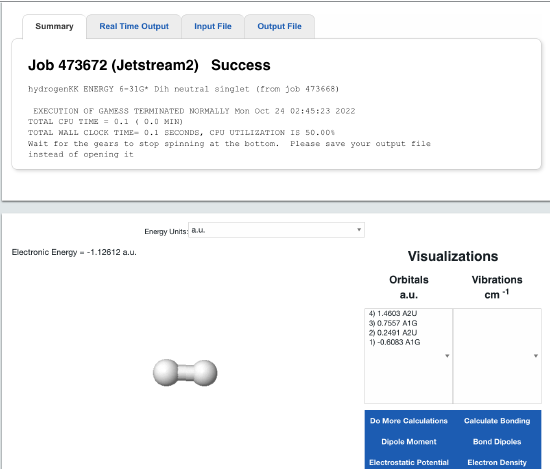
There are many interesting aspects to this calculations, but for now, we are focusing on the "Electronic Energy" right above the molecule. Later on we will review the (molecular) orbitals and other cool things you can calculate. Set the energy units to kcal/mol (right above the molecule).
Build the Potential V(x)V(x) for H2H2 Vibration
Construct the potential curve for molecular hydrogen one geometry point at a time (this is the Born-Oppenheimer approximation). This is a potential without any approximations such as the harmonic or anharmonic oscillator potential. It is a numerical potential and is inserted into the vibration Schrödinger equations to solve for the wavefunctions and energies via numerical approaches.
To do this you must vary the bond length. From the output of your job do this by:
- Note the electronic energy (change the units to kcal/mol)
- Click "Do More Calculations"
- Click "Manually alter coordinates"
- Double check the bond length for this calculation (calculate the distance between the two atoms)
- Vary the distance between the two atoms by editing the coordinates. It's easiest to place one atom at the origin.
- Check "Single-Point Energy" next to "Type of Calculation" This will instruct GAMESS not to change your coordinates.
- Click "Create Input File"
- Click "Submit Job"
- When the job is finished ("Success") repeat from step 1
For each bond length you will enter the electronic energy in the following table:
| Bond Length (Angstroms) | Energy (Kcal/mol) for H2H2 |
|---|---|
| 0.2 | 48.99 |
| 0.25 | |
| 0.3 | |
| 0.35 | |
| 0.4 | |
| 0.5 | |
| 0.6 | |
| 0.7 | |
| 0.8 | |
| 0.9 | |
| 1.0 | |
| 1.1 | |
| 1.2 | |
| 1.3 | |
| 1.4 | |
| 1.5 | |
| 2 | |
| 3 | |
| 4 | |
| 5 | |
| 6 | |
| 7 |
To be Submitted for Credit:
- Submit the above table filled out for the electronic energy of each bond length
- Plot up this potential energy curve on your favorite software (E.g., excel or desmos or matlab or matplotlib)
- From this plot, answer these two questions:
- What is the equilibrium bondlength for H2H2?
- What is the bond energy (well depth) for H2H2?
Optional:
Try to fit a parabolic potential (i.e., a quantum Harmonic Oscillator or anharmonic Morse potential) to the experimental curve and extract a "spring constant" for this vibration.

