3: Solutions

This Lab will have four parts

Part 1: Upload a hand written graph of last week's lab to a Google Doc using a scanner or the Genius Scan cellphone app.

Part 2: Analyzing some experimental issues.

Part 3: Drawing a solubility curve for an unknown in a virtual lab

Part 4: Solubility Conversions

Review of Last Week

In last weeks lab you used a spreadsheet (Google sheets) and plotted solubility data from two salts, of KI and one of KNO₃. This week you need to demonstrate that you can do this by hand, without a graphing program.  Last week you plotted two sets of data; one plot linear, the other was not. Subsequently you ran fitting programs to fit the nonlinear graph to a power function and an exponential function. After that you created a log [concentration] vs. log [T] plot that you related to the power function, and then a ln [concentration] vs. T plot and related that to the exponential function. Your first activity is to create a hand written graph of either the log/log plot or the ln plot. First, lets revisit some issues we had last week.

Issue 1: Plotting the log of Zero.  Last week when you used your calculator (or an equation in google sheets) to calculate the log of zero it gave an error.  Why?  Well the log of a number is 10 to a power that equals that number.  So log 100 = 2 because 10² = 100 and log(\(\frac{1}{100}\)) = log0.01= -2 because 10^-2 = 0.01, or a tenth of a tenth (one hundredth).  So if every time you divide by 10 you reduce the prior value, you would need to divide an infinite number of times to hit zero.

\[0=\frac{1}{10^{\infty}} =10^{-\infty} =0 \\  \text{ so log0 =  }-\infty\]

(no wonder your calculator gives an error)

Issue 2: Which plot was the best?

S=AT^m    or    S=Ae^mT

where S= solubility and T=temperature (note, we use T for temperature, and t for time).

You may look at the R² value from Excel or Google Sheets, which is the "coefficient of determination" and describes the variation of the data from your plot.  The value ranges from 0 to 1, with 1 being the best fit.  But statistics only goes so far, and one of these two equations makes no sense, even if it has the best fit.  Can you guess which one it is, and why?

Well, lets look at the power function, and say we are using the Celsius temperature scale. Well there are two issues, first, it says salt can not dissolve in water at zero Celsius, as no matter what the value of m, 0^m= 0 and well, that is simply not true, and you can have salt water at its freezing point (as long as it is not ice). The second thing that makes no sense is if you change the scale to Fahrenheit, where the freezing point is 32^oF, well, it an suddenly dissolve salt? 

Issue 3: Solubility is a Bounded Function

This is a science class and not a math class, and you need to realize that these equations are a form of language that describes the temperature dependence of the solubility of a salt in water, and implicit in that is the fact that you have liquid water. So this equation if only valid over the range of temperature where liquid water exists and is not valid for ice or steam. Of interest, as we shall see, a solute actually lowers the freezing point and raises the boiling point.

 

Part I Hand Written Graph

In general chemistry 1 students usually do a hand written graph and this was skipped this year, and so we are going to pick it up now. In this activity you will learn how to take the solubility data of KNO₃ and determine the value of A and m by hand for an exponential fit, S=Ae^mT.  Using the  KNO₃ data from Experiment 2 and using a calculator convert the solubility data to natural log (ln) and plot the lnS (dependent variable) as a function of the T (independent variable).  From the slope of the line and the Y-intercept you can then calculate A and m for the exponential equation without using a spreadsheet.  This values should correlate to the last graph of experiment 2.

Go to Google Classroom and do Part 1 of experiment 3, following these guidelines

Supplies

To do this you will need to get some graph paper and have access to a cell phone or a scanner

Graph Paper: and please contact your instructor if you do not have a cell phone or scanner.  If you do not have access to any graph paper you can either download and print it, or make your own with a ruler.  A google search of free printable graph paper will give many options, including this one, https://www.vertex42.com/Files/pdfs/2/printable-graph-paper_10x1-inch.pdf

Scanner/Genius Scan App: If you have a scanner you can use that, if not, go to appendix 1, download the genius scan app and follow instruction on how to use it.  It may be easiest to scan your graph paper, upload it to your computer and display the image on your computer, and then use the snipping tool to crop it and place it into the Google doc.

 

Steps for Graphing a Linear Function

1. Pick your range and scale: In graphing a linear function the first step is to identify the range and scale for each axes. The range is defined by the minimum and maximum value along each of the axes. The scale is defined by the values of each line in the grid, which is used both to plot the data points, and once graphed, to read values from the graph. There are often minor and major marks given to the grid, where the major marks show the numerical value of that position.

• Choosing the Range: There are two approaches. The first is to use the highest and lowest data value as the lower and upper bound of the range, although you may want the actual bounds to be some easy number to read, like a multiple of ten. The second approach is to look at the data, and see if the data is bounded by some real limit. For example, in the above data we are looking at the solubility of a salt in liwuid water, so the temperature range may want to be defined by the temperature range where water is a liquid, even if your highest data point is not at the boiling point, and your lowest is not at the freezing point.
• Choosing the Scale: Here you want the grid line to be easy to read. If possible, multiple's of 10 are very useful, but you need to look at the data. Want you want to avoid is where each mark is some hard to read value.

2. Plot data: Mark each data point on the graph (like in Figure 1B.5.1, but do not write down the x,y coordinate values, just mark a point on the graph to indicate where there is a data value.
3. Hand draw a best fit line that has an even distribution of points on both sides of the line. If the data is truly a linear function, there will be a random distribution of points along the line. Figure 1b.5.3 shows such a "best fit line".
4. 
   
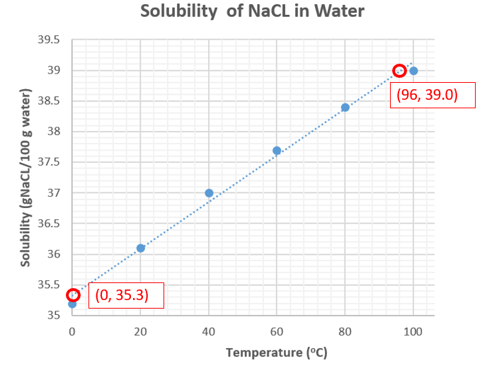
   Figure \(\PageIndex{1}\): Best fit line that evenly describes the data. Not we do not connect the points, and some of the points are not on the line.
    
5. Pick two points to calculate the slope from. Start at the left side and find the point on the line with the smallest values where the line crosses the grid lines, here it is point (0,25.50), and then starting at the right end pick the point with the highest values (96,39.00).

• Note the precision is defined by both the data and the scale on the grid lines.
  • For the y-axis the precision is defined by the data, and although we have a mark every 0.1 values, so it looks like we could report solubility to the .01 value, the original data was only known to the 0.1 value (table 1B.5.1). So so even though the scale on the graph is more precise, we can only use that precision to read from the scale, and not report the value. That is from the scale we could read to a value of 35.30 and not 35.3, but we must use 35.3 in our calculation
  • For the x-axis the original data has a precision to the 0.1 digit, that is, we have values like 20.0 ^oC. But the smallest value on the minor grid axis is 4 ^oC, and so we have to "guess" between them to report the uncertainty, and thus choose the precision to be to the "ones" position.
• Note, if we choose points near to each other, we can lose significant digits. For example, if the second point was (4,35.5) the change in temperature would be 4-0 or 4 degrees (1 significant digit), while using the value on the graph give 96-0, or 96 degrees, which has two significant Figures.
• That is, we report all certain, and the first uncertain data point, as read off the graph. A graph scale should never have a smaller scale than the raw data, that is, it can't add to the precision

5. Now calculate the slope
   
   \[\text{slope} = m=\frac{\text{rise}}{\text{run}} = \frac{\left( y_2 - y_1 \right)}{\left( x_2 - x_1 \right)} =\frac{\left( S_2 - S_1 \right)}{\left( T_2 - T_1 \right)} =\frac{\left( 39.0 -35.3 \right)}{\left( 96 - 0 \right)} = {\color{blue}0.039 \:\frac{g\; NaCl}{100gH_2O\cdot \; ^oC}}\]
6. Now calculate the y intercept. Since the graph goes through zero, you can just read it from the graph

• Since the x-axis includes zero, you can simply read it from the graph, b=35.3(gNaCl/100g water).
• If your graph does not include the zero point, you can extrapolate backwards from a given value.
  We know that:

  \[m=\frac{\Delta{y}}{\Delta{x}} = \frac{\Delta{S}}{\Delta{T}} \]

If we define S₂₀=solubility when T=20, and S₀=solubility when T=0, then b= S₀, and S₂₀ comes from the graph on Figure 1B.5.3 where, S₂₀=36.1(gNaCl/100g water).

\[{\color{blue}m}=\frac{\textcolor{red}{S_{20}}-S_{0}}{20-0}= \frac{\textcolor{red}{S_{20}}-b}{\Delta{T}_{(=20)}}\]

Where \(\Delta{T_{(=20)}}\) means the value of \(\Delta T\)= 20,

solving for b and including units in numerical calculation gives:

\[b={\color{Red} S_{20}}-\textcolor{blue}{m}(\Delta{T}_{(=20)})={\color{red}36.1\left (\frac{g\; NaCl}{100gH_2O} \right )}- {\color{blue}0.039 \:\frac{g\; NaCl}{100gH_2O\cdot \; ^oC}}\left ( 20 \; ^oC\right )=35.3\left (\frac{g\; NaCl}{100gH_2O} \right )\]

 

 

 

Part II: Different units of concentration

Chemists need to be able to make and deliver solutions of different concentrations and we will use various quantitative measuring devices like a Buret, Pipet, Volumetric Flask and a Graduated Cylinder.  Each instrument has a defined precision that is based on how precisely it was calibrated.  In this class, we will use the values that are given in figure \(\PageIndex{2}\), which are typical for instruments in a university lab, and so if we say "dilute to volume in a 50 ml volumetric flask" you need to know that number has 4 significant digits.  Now realize in a real lab you need to look at the actual device you are using to identify its precision, which may vary from the ones we are using in this lab. 

 

Figure \(\PageIndex{2}\): Precision of common volumetric measuring Devices.

What you will notice in Figure \(\PageIndex{2}\) is that some of the devices are labeled TC (to contain) and others a labled TD (To Deliver).  If a graduated cylinder is labeled TD then it is calibrated to deliver a the defined amount of fluid, and you do not have to worry if some of the fluid sticks to the side, but if it is labeled TC and you want to transfer the exact amount you measure, you have a problem.  A volumetric flask is labeled TC and if you dilute it to the mark you have created a solution of the defined volume of the flask.  

Making a Solution from a solid solute

The first step to making a solution is to weight the solute.  To do this you first tare of the weight of the weighing paper or boat (figure ) and then accurately record the weight of the solute.  You then quantitatively transfer it to a volumetric flask of the desired volume, rinsing any solute that may be on the funnel to make sure it is all transferred and then add water until it is about half full.  Then you mix the solution until it is all dissolved and at the final stage you dilute with solvent until the bottom of the meniscus touches the calibration mark.  You know need to either stopper the flask and invert several times to ensure mixing.

Figure \(\PageIndex{3}\): First calculate the approximate mass of reagent you need to dilute to the desired concentration.  If it is a hydrated salt you include the water of hydration, the example here is of copper(II) nitrate hemi(pentahydrate), Cu(NO₃)₂^.2.5H₂O, which has a molar mass of 232.59g/mol and we wish to make 1 liter of 0.2M solution.  This is an approximate mass, and we will determine the final concentration based on the actual mass transferred.

Figure \(\PageIndex{4}\): We then tar of the weight of the weighing paper or boat.  Note how we folded the weighing paper so it can easily pour the solute into the flask

Figure \(\PageIndex{5}\): We now weigh the desired mass and record the actual mass transferred.  Do not put more solute on the weighing paper than can be safely handled and transferred, and be sure all the solute is transferred to the desired volumetric flask. In this case we are going to transfer the solute in two steps as 96 grams is too much to place on one piece of weighing paper.

Figure \(\PageIndex{6}\): When transferring to a narrow mouthed volumetric flask you should use a funnel, and be sure to rinse any solute that may stick to the side of the funnel.

 

 

Figure \(\PageIndex{7}\): Fill the volumetric flask half way and swirl around until all the solute is dissolved.  You must dissolve all the solute or you can not calculate the concentration. 

Figure \(\PageIndex{8}\): After all the solid solute dissolves dilute to volume

Figure \(\PageIndex{9}\): Make sure your eye is parallel to the calibration mark when you make the final determination and the bottom of  the meniscus should just touch the mark.

Figure \(\PageIndex{10}\): Place the cap on the volumetric flask and invert several times to ensure thorough mixing, or as in this image, you can add a magnetic stirring bar, after you have diluted to volume.  You are now ready to calculate the final concentration based on the actual mass you added, and report it to the correct number of significant digits.

 

Student Activity

In this activity you will use a Google sheet to calculate the concentration of a salt in different units.  In this activity a student will measure the mass of a salt using either a 25, 50  or 100 ml flask, then add some salt and reweigh, and finally dilute to volume and weigh the mass of the flask and solution.

Note, a 25 ml flask is known to the precision the volumetric flasks are given in figure 3 and you must report your answers to the correct number of significant digits.  The Google sheet will let you check your work for mathematical correctness, but not for significant digits.

Values of Student Unknowns

Unknown	A	B	C	D	E	F
Salt Identity	Sodium Nitrate	Potassium Nitrate	Sodium Chloride	Calcium Chloride	Sodium Sulfate	Lithium carbonate
Mass Volumetric Flask (g)	25.0124	40.0993	25.8392	39.6291	24.9483	40.0382
Mass Volumetric Flask + Salt (g)	26.3048	42.0995	28.2938	44.3727	27.3948	43.0637
Mass Volumetric Flask + Salt + Water  (g)	51.0483	91.8923	57.4439	93.8382	52.2894	92.3863
Size Volumetric Flask (ml)	25	50	25	50	25	50

 

Students will then input the data in their Google Sheet as described in figure \(\PageIndex{11}\).

Figure \(\PageIndex{1}\): Google worksheet where each student submits answers in a separate tab. (Belford/Poirot)