6.3: Atomic Line Spectra and Niels Bohr

Learning Objectives 

• Define the ground state ground state and excited state of electrons 
• Explain the difference between line spectra for absorption and emission of electrons
• Calculate the energy associated with the electron at specified energy state
• Calculate the energy difference with electron transition from a higher energy to lower energy, and vice versa
• Calculate the wavelength of light emitted as a result of a particular energy transition 
• Differentiate between the Balmer, Lyman, and Paschen Series 
• Describe the limitation of the Bohr Model 

Line Spectra

In a gas discharge tube energy is added to a gas which is adsorbed by electrons. These excited electrons then fall back to their lower energy and can give off a photon of light of a specific wavelength that can be seen by splitting the emitted light beam through a diffraction grating or prism. These type of spectra are called line spectra (in contrast to continuous spectra like the colors of the rainbow) and each element has a unique line spectra that can be used to identify it.

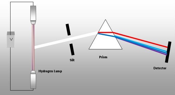
Fig. 6.3.1 Prism showing light being emitted from hydrogen being separated into discrete wavelengths (colors), in contrast to the continuum of white light, as in the rainbow.

In understanding the following line spectra we need to realize that when a photon of light has the energy of the gap between to orbitals, it can allow an electron to jump from one orbital to another. There are two possibilities, it could jump to a higher energy orbital (absorption), or relax to a lower energy orbital (emission).

Fig. 6.3.2 Hydrogen Emission Spectra as would be observed with a gas discharge lamp.

Note that only light of specific frequencies (the lines) are observed, which is why we call it a line spectra. Each element would give a unique line spectra, and like a fingerprint, these can be used to identify the elements in a gas. This spectra is created by exciting hydrogen gas so electrons enter excited states, as in fig. 6.3.1. The electrons then relax back to the ground state through both radiative and nonradiative processes, with the radiative processes emitting photons that correlate to the energy gap between an excited and lower energy orbital. The black region represents colors of energy where there is no gap between electron orbitals that can radiate.

Fig. 6.3.3 Hydrogen Absorption Spectra, as would be observed if a continuous spectra was passed through hydrogen gas that was not excited. (Hitting the prism in figure 6.3.1 with white light, and placing the gas on the other side. )

Here the black bands indicate light of an energy where electrons in the hydrogen could absorb it by jumping to a higher energy state, and so that light was not transmitted through the sample but absorbed. The colored background is light that was transmitted through the sample because there was no allowed transition where the energy gap between two orbitals equaled the energy of the photon (h\(\nu\)) .

Balmer Equation

Based on empirical data measured by Anders Angstrom, Johann Balmer (1825- 1898) was a Swiss mathematician who developed an equation for computing the wavelengths of the line spectra. It needs to be emphasized that although this equation could account for the line spectra it was based on empirical (experimental) data.

\[\lambda =B\left ( \frac{n^{2}}{n^{2}-2^{2}} \right )\]

Balmer Equation describing the visible spectrum for hydrogen atom, where B = 364.56 nm, and n is an integer larger than 2.

Rydberg Equation

Johannes Rydberg came up with a more general equation of which the Balmer equation is a specific example for n

\[\frac{1}{\lambda }=R\left(\frac{1}{n_{1}^{2}}-\frac{1}{n_{2}^{2}}\right)\]

R is the Rydberg constant, R= 1.097x10⁷m^-1 and n₁<n₂. The following image shows the line spectra in the ultraviolet (Lyman series), visible (Balmer series) and various IR series that are described by the Rydberg equation.

Algebra challenge, show that the Balmer Equation is a special instance of the Rydberg equation where n₁=2, and show that B = 4/R. In the next section we will look at the Bohr model, and derive a form of the above equation from an energetics perspective.

The following video explains the Balmer and Rydberg equations

https://youtu.be/WEh2LEulw1w Please note, this video goes in and out of focus and needs to be redone, as the camera needs to have autofocus turned off.

Bohr Model

The Bohr model provides a theoretical framework for understanding line spectra. If a photon of light is absorbed its energy (h\(\nu\)) is transferred to an electron which jumps from a low energy orbit to a high energy orbit, and the absorption spectral lines are correlated to wavelengths associated with the frequency of that light (C=\(\lambda \nu\)). In an emission spectra electrons are excited to upper energy states by some external energy source (thermally or electronically like in a discharge lamp), and then the excited electron spontaneously falls back to the lower energy ground state. This may happen through thermal or radiative means, and if it occurs through a radiative process, a photon of the energy associated with the electronic transition is emitted and this accounts for the lines in an emission spectrum. It is important to recognize that absorption is an endothermic process where the atom gains the energy of the photon, and emission is an exothermic process where the atom losses the energy of the emitted photon.

The Bohr model is actually very simple to understand, in that it states the energy of the nth orbital is quantized, and inversely related to the square of the quantum number (n) times the energy required to ionize the electron, that is, to remove it from an orbit. This is described by the following equation and the reason it is negative is because zero energy is that when the electron and proton are separated by infinity, and noting that to remove an electron is an endothermic process (you add energy), means the energy of an electron in an orbital must be less than zero..

\[E_{n}=-R_{\infty}\left(\frac{1}{n^{2}}\right)\]

Note: The above equation is a form of an inverse square law, except that unlike other inverse square laws, it is based on the value of an integer, \(\frac{1}{n^{2}}\), giving it values of 1,1/4,/1/9,/16,1/25...

Other inverse square laws are like Coulomb's Law, \(F=k\frac{Q_{1}Q_{2}}{r^{2}}\) and Newton's Law \(F=G\frac{m_{1}m_{2}}{r^{2}}\) . The difference is that the Bohr model is treating energy as a series of discrete (quantized) values inversely proportional to an integer, while Coulomb's and Newton's Law relates the force to the inverse square of the distance between two interacting particles, and is a continuum. That is, unlike Bohr's model, the particles can be separated by any distance (r is not restricted to discrete values).

\[E_{electron}= \Delta E_{n_{i}\rightarrow{n_{f}}}=E_{n_{f}}-E_{n_{i}}=-R_{\infty}\left(\frac{1}{n_{f}^{2}}-\frac{1}{n_{i}^{2}}\right)\]

\[E_{photon}=h\nu =\frac{hc}{\lambda }\]

Absorption Spectrum

(this is endothermic and n_f > n_i)

The energy of the photon equals the energy of the electron transition as it absorbs the energy and goes to a higher level.
\[E_{photon}=E_{electron}\]
substituting \[h\nu =E_{n_{f}}-E_{n_{i}}\]
\[\frac{hc}{\lambda }=-R_{\infty}\left(\frac{1}{n_{f}^{2}}-\frac{1}{n_{i}^{2}}\right)\]
Noting \(R_{\infty}\) is the minimum energy required to photo-ionize an electron in the lowest energy level, that is, to eject the electron from hydrogen so it is not longer in an orbital.

\[\frac{hc}{\lambda }=-R_{\infty}\left(\frac{1}{n_{f}^{2}}-\frac{1}{n_{i}^{2}}\right)\]

To derive the Rydberg Equation we first divide by hc

\[\frac{1}{\lambda }=-\frac{R_{\infty}}{hc}\left(\frac{1}{n_{f}^{2}}-\frac{1}{n_{i}^{2}}\right)\]

Then multiply by negative one
\[\frac{1}{\lambda }=\frac{R_{\infty}}{hc}\left(\frac{1}{n_{i}^{2}}-\frac{1}{n_{f}^{2}}\right)\]

And equate the Rydberg constant to \(R_{\infty}\)/hc
\[\frac{1}{\lambda }=R\left(\frac{1}{n_{i}^{2}}-\frac{1}{n_{f}^{2}}\right)\]

Note R = 1.097x10⁷m^-1
and is the historical Rydberg constant that predicted the wavelength of the hydrogen spectra.

What we are calling \(R_{\infty}\) is the minimum energy required to remove an electron from the ground state (lowest energy) orbital of hydrogen, and
\(R_{\infty}\) = 2.18x10^-18J

noting that

\[R=\frac{R_{\infty}}{hc}\]

so to relate the Rydberg constant to the energy required to completely remove an electron (R_\(\infty\)), that is, R

TAKE HOME:

If you are given R = 1.097x10⁷m^-1 use:
\[\frac{1}{\lambda }=R\left(\frac{1}{n_{i}^{2}}-\frac{1}{n_{f}^{2}}\right)\]

If you are given R = 2.18x10^-18J, use
\[\frac{1}{\lambda }=-\frac{R}{hc}\left(\frac{1}{n_{i}^{2}}-\frac{1}{n_{f}^{2}}\right)\]

Bohr Model and Line spectra

7:02 YouTube showing how you can use the Bohr model to determine the line spectra of hydrogen.

Emission spectrum

the system loses an energy as the photon is leaving (exothermic) and so the energy is negative (n_i > n_f)

\[-E_{photon}=E_{electron}\]

\[-\frac{hc}{\lambda }=-R_{\infty}\left(\frac{1}{n_{f}^{2}}-\frac{1}{n_{i}^{2}}\right)\]
Noting \(R_{\infty}\) is the minimum energy required to photo-ionize an electron in the lowest energy level, that is, to eject the electron from hydrogen so it is not longer in an orbital.

\[\frac{hc}{\lambda }=R_{\infty}\left(\frac{1}{n_{f}^{2}}-\frac{1}{n_{i}^{2}}\right)\]

To derive the Rydberg Equation we first divide by hc

\[\frac{1}{\lambda }=\frac{R_{\infty}}{hc}\left(\frac{1}{n_{f}^{2}}-\frac{1}{n_{i}^{2}}\right)\]

or

\[\frac{1}{\lambda }=R\left(\frac{1}{n_{f}^{2}}-\frac{1}{n_{i}^{2}}\right)\]

 

Example \(\PageIndex{1}\)*

The so-called Lyman series of lines in the emission spectrum of hydrogen corresponds to transitions from various excited states to the n = 1 orbit. Calculate the wavelength of the lowest-energy line in the Lyman series to three significant figures. In what region of the electromagnetic spectrum does it occur?

Solution

Given: lowest-energy orbit in the Lyman series

Asked for: wavelength of the lowest-energy Lyman line and corresponding region of the spectrum

Strategy:

A Substitute the appropriate values into Equation 2.5.2 (the Rydberg equation) and solve for λ.

B Use Figure 2.5.1 to locate the region of the electromagnetic spectrum corresponding to the calculated wavelength.

Solution:

We can use the Rydberg equation to calculate the wavelength:

\( \dfrac{1}{\lambda }=-\Re \left ( \dfrac{1}{n_{2}^{2}} - \dfrac{1}{n_{1}^{2}}\right ) \)​

A For the Lyman series, n₁ = 1. The lowest-energy line is due to a transition from the n = 2 to n = 1 orbit because they are the closest in energy.

\( \dfrac{1}{\lambda }=-\Re \left ( \dfrac{1}{n_{2}^{2}} - \dfrac{1}{n_{1}^{2}}\right )=1.097\times m^{-1}\left ( \dfrac{1}{1}-\dfrac{1}{4} \right )=8.228 \times 10^{6}\; m^{-1} \)

It turns out that spectroscopists (the people who study spectroscopy) use cm^-1 rather than m^-1 as a common unit. Wavelength is inversely proportional to energy but frequency is directly proportional as shown by Planck's formula, E=h\( \nu \). Spectroscopists often talk about energy and frequency as equivalent. The cm^-1 unit is particularly convenient. The infrared range is roughy 200 - 5,000 cm^-1, the visible from 11,000 to 25.000 cm^-1 and the UV between 25,000 and 100,000 cm^-1. The units of cm^-1 are called wavenumbers, although people often verbalize it as inverse centimeters. We can convert the answer in part A to cm^-1.

\( \varpi =\frac{1}{\lambda }=8.228\times 10^{6}\cancel{m^{-1}}\left (\frac{\cancel{m}}{100\;cm} \right )=82,280\: cm^{-1} \)

and

λ = 1.215 × 10⁻⁷ m = 122 nm

This emission line is called Lyman alpha. It is the strongest atomic emission line from the sun and drives the chemistry of the upper atmosphere of all the planets producing ions by stripping electrons from atoms and molecules. It is completely absorbed by oxygen in the upper stratosphere, dissociating O₂ molecules to O atoms which react with other O₂ molecules to form stratospheric ozone

B This wavelength is in the ultraviolet region of the spectrum.

 

Exercise \(\PageIndex{1}\)*

The Pfund series of lines in the emission spectrum of hydrogen corresponds to transitions from higher excited states to the n = 5 orbit. Calculate the wavelength of the second line in the Pfund series to three significant figures. In which region of the spectrum does it lie?

Answer

4.65 × 10³ nm; infrared

 

Limitation of the Bohr Model 

Although Bohr introduced the idea of a quantization to the way we describe an atom by validating something that he had no of seeing (structure of the atom) and tying it into experimental results that he observed (spectra) through a mathematical equation, his theory was incomplete. As a matter of fact, it could only explain the structure of atoms with only one electron like hydrogen or He⁺. When more than one electron was involved in atom, there was no model to explain the spectra. So, a better model was needed that was all encompassing. 

 

Extra Practice

• CHEMTOUR - Click Ch 7: "Light Emission and Absorption" and "Bohr Model of the Atom"
• Self Quiz : Click Electronic Transitions for Hydrogen  and Electronic Transitions for Hydrogen-like Species
•  

Contributors 

• Robert Belford (UA of Little Rock) 
• Modified by Ronia Kattoum (UA of Little Rock) 
• *Original Source of Example and Exercise 1