5.6: Calorimetry

Learning Objectives 

• Apply the First Law of Thermodynamics to calorimetry 
• Compare heat flow from hot to cold objects in an ideal calorimeter versus a real calorimeter 
• Calculate heat, temperature change, and specific heat after thermal equilibrium is reached between two substances in a calorimeter
• Calculate the molar heat of enthalpy for a reactions using coffee cup calorimetry
• Compare and contrast coffee cup calorimetry and bomb calorimetry

Calorimetry

Calorimetry is an application of the First Law of Thermodynamics to heat transfer, and allows us to measure the enthalpies of reaction or the heat capacities of substances. From the first law we can state

Δ E_Universe = Δ E_System + Δ E_Surrounding = 0

therefore,

Δ E_System = -Δ E_Surrounding

A calorimeter is an instrument that has a thermally isolated compartment that is designed to prevent heat flow to the surroundings. Technically, this is called an adiabatic surface in that no heat flows in and out of the calorimeter, which is in contrast to isothermal, which means constant temperature. In truth, there is no such thing as a thermally isolated system, but we can design systems that approach it on the time scale of a measurement. We will consider two types of calorimeters, ideal calorimeters, where the calorimeter does not absorb heat itself, and real calorimeters, where the calorimeter and it's contents absorb heat. We will apply calorimetry to two different thermodynamic processes, that of transference of heat across objects at different temperatures, and that released or absorbed by a chemical reaction. We will look at two ways of measuring this heat, either the temperature change of the calorimeter, or the mass of a substance that undergoes a phase change within the calorimeter at a constant temperature.

If we consider the work in a calorimeter to be zero, and noting that Δ Q + W, the above equation becomes

Q_System = -Q_Surrounding

If we can measure the heat absorbed or lost by the surroundings we can use the above equivalence statement to calculate the heat lost or absorbed by the system, and this is the basis for calorimetry,

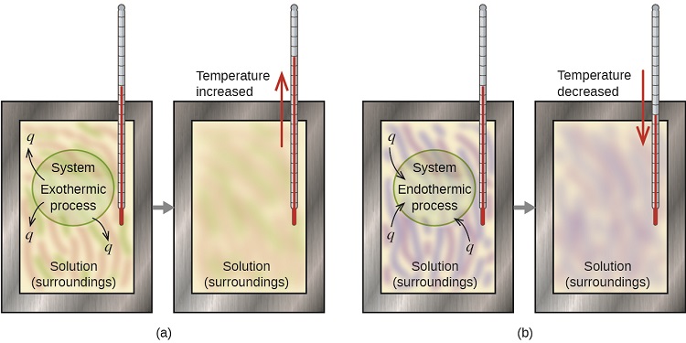
Figure 5.6.1: In part a, and exothermic process occurs and the calorimeter's temperature rises, while in part b an endothermic process occurs and the temperature falls.

 

Heat Transfer Between Hot and Cold Objects in an Ideal Calorimeter

When a hot object (T_H) is placed in thermal contact with a cold object (T_C) energy is transferred between the two, but the rate of heat transfer from the hot to the cold is greater, so it cools down while the cold object heats up, until they reach the same temperature (T_F). Once they are at the same temperature the system is at thermal equilibrium and the rate of transfer of energy from the hot to cold is the same as cold to hot. That is, energy is a vectoral flow, and even at the same temperature, there is a flow of energy across the boundary of two objects, but the flow is the same.

Fig 5.6.2, Graph showing temperature change as a function of time after a hot object is put in thermal contact with a cold object. Note, that in this case the capacity of the cold object to hold heat is greater, so the change in temperature of the cold object is less than the hot. Also note, ΔT = T_Final - T_Initial and ΔT_Hot is a negative number (it cools, so T_F < T_i ) while ΔT_Cold is a positive number, (it heats, so T_F > T_i ).

 

When two objects at different temperatures are placed in contact, heat flows from the warmer object to the cooler one until the temperature of both objects is the same. The law of conservation of energy says that the total energy cannot change during this process:

\[q_{cold} + q_{hot} = 0 \label{12.3.9}\]

The equation implies that the amount of heat that flows from a warmer object is the same as the amount of heat that flows into a cooler object. Because the direction of heat flow is opposite for the two objects, the sign of the heat flow values must be opposite:

\[q_{cold} = −q_{hot} \label{12.3.10}\]

Thus heat is conserved in any such process, consistent with the law of conservation of energy.

The amount of heat lost by a warmer object equals the amount of heat gained by a cooler object.

Substituting for \(q\) from Equation 1 gives

\[ \left [ mc_s \Delta T \right ] _{cold} + \left [ mc_s \Delta T \right ] _{hot}=0 \label{12.3.11}  \]

which can be rearranged to give

\[ \left [ mc_s \Delta T \right ] _{cold} = - \left [ mc_s \Delta T \right ] _{hot} \label{12.3.12} \]

When two objects initially at different temperatures are placed in contact, we can use Equation \(\ref{12.3.12}\) to calculate the final temperature if we know the chemical composition and mass of the objects.

 

Example \(\PageIndex{1}\): Thermal Equilibration of Copper and Water

If a 30.0 g piece of copper pipe at 80.0°C is placed in 100.0 g of water at 27.0°C, what is the final temperature? Assume that no heat is transferred to the surroundings.

Given: mass and initial temperature of two objects

Asked for: final temperature

Strategy: Using Equation \(\ref{12.3.12}\) and writing \(ΔT= T_{final} − T_{initial}\) for both the copper and the water, substitute the appropriate values of \(m\), \(c_s\), and \(T_{initial}\) into the equation and solve for \(T_{final}\).

Solution

We can adapt Equation \(\ref{12.3.12}\) to solve this problem, remembering that \(ΔT= T_{final} − T_{initial}\):

\[ \left [ mc_s \left (T_{final} - T_{initial} \right ) \right ] _{Cu} + \left [ mc_s \left (T_{final} - T_{initial} \right ) \right ] _{H_{2}O} =0 \]

Substituting the data provided in the problem and Table \(\PageIndex{1}\) gives

\[\begin{align*} \left (30 \; g \right ) (0.385 \; J/ (g °C) ) (T_{final} - 80°C) + (100\;g) (4.184 \; J/ (g °C) ) (T_{final} - 27.0°C ) &= 0 onumber \\[4pt] T_{final}\left ( 11.6 \; J/ ^{o}C \right ) -924 \; J + T_{final}\left ( 418.4 \; J/ ^{o}C \right ) -11,300 \; J &= 0 \\[4pt] T_{final}\left ( 430 \; J/\left ( g\cdot ^{o}C \right ) \right ) &= 12,224 \; J  \\[4pt] T_{final} &= 28.4 \; ^{o}C \end{align*} \]

 

Example \(\PageIndex{2}\)

 What is the final temperature when 2.00 g of gold at 100°C is placed into 25.0 mL of water at 30.0°C? 

Solution

Video Tutor:

 

 

 

Exercise \(\PageIndex{1}\): Thermal Equilibration of Gold and Water

If a 14.0 g chunk of gold at 20.0°C is dropped into 25.0 g of water at 80.0°C, what is the final temperature if no heat is transferred to the surroundings?

Answer

80.0°C

 

 

 

 

 

 

 

 

 

 

 

 

 

 

 

 

 

 

 

 

 

 

 

 

 

 

 

 

 

 

 

Exercise \(\PageIndex{2}\)

28.0 g chunk of aluminum is dropped into 100.0 g of water with an initial temperature of 20.0°C. If the final temperature of the water is 24.0°C, what was the initial temperature of the aluminum?  (Assume that no heat is transferred to the surroundings.)

Answer

90.6°C

 

 

Heat Transfer Between Hot and Cold Objects in a Real Calorimeter

In a real calorimeter the calorimeter itself will absorb some of the heat, even if it transfers no heat to the surroundings. That is, the calorimeter itself has a heat capacitance. This usually needs to be measured for each calorimeter, and following the conventions of section 4.2, we use a capital C to represent the capacitance of an object, or the calorimeter constant. That is, the calorimeter constant is the calorimeter's heat capacitance.

If as in the above case we add a hot object to water in a calorimeter, both the water and the calorimeter are heated. Starting with the First Law (and considering work to be zero), we have

Q_Cold = -Q_Hot 

But now there are two cold objects, the water and the calorimeter, so

Q_Cold = m_cc_cΔT_c + C_cΔT_c , where

m_c = mass cold water
c_c = specific heat capacity of water (m_cc_c is the heat capacitance of the water in the calorimeter)
C_c = calorimeter constant
ΔT_C = T_F - T_C

Substituting give

m_cc_cΔT_c + C_cΔT_c = m_Hc_HΔT_H , which can be rearranged to

(m_cc_c + C_c)ΔT_c = m_Hc_HΔT_H

 

Example \(\PageIndex{3}\)

If 150 g of lead at 100.0°C were placed in a calorimeter with 50 g of water at 22.0°C and the resulting temperature of the mixture was 26.2°C, calculate the q_cal, q_H20, q_Pb? The specific heat of water is 4.184 J/g °C and the specific heat of lead is 0.128 J/g °C.

Solution

For lead, we know that:

m(mass) = 150 g,
T_i (initial temperature) = 100.0°C
T_f = 26.2°C
c_sp (specific heat of lead) = 0.128 J/g °C

For water:

m= 50 g,
T_i = 22.0°C
T_f = 26.2°C
c_sp = 4.184 J/g °C

\[q =m\, csp \, \Delta T \]

q_Pb = (0.128 J/g °C )(150 g ) (26.2°C - 100°C) = -1.42 x 10³ J

qH₂O= (4.184J/g °C)(50 g) (26.2°C - 22°C) = 8.79 x 10² J 

q_cal + q_Pb + q_H20 = 0 

q_cal = -(q_Pb + q_H2O) 

q_cal = -(-1.42 x 10³ J +  8.79 x 10² J ) = 541 J 

This would be mean that 541 J of heat were absorbed by the calorimeter (in addition to what was absorbed by the water). 

 

Exercise \(\PageIndex{1}\)

For Example 3, calculate the calorimeter constant (C_c) for that particular calorimeter that was used to collect the data:

Answer

 

Exercise \(\PageIndex{2}\)

Do you think the final temperature will be higher or lower for the problem in the video of cooling 2.00 g of gold in water if we include the calorimeter constant in the equation?

Answer

It will be cooler, as there are two things being heated, the water and the calorimeter itself. 

 

Constant Pressure Calorimetry, Measuring Enthalpy

We have seen how we can measure heat flow from a hot object to a cold object using Calorimeters. Calorimeters can also measure the molar enthalpy of reaction, by simply equating the heat absorbed/lost by the calorimeter to the heat lost/absorbed by the reaction. That is, the system is the reaction. In the laboratory, we often use a simple device that is called the coffee cup calorimeter. 

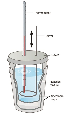
Figure \(\PageIndex{3}\): A simple calorimeter can be constructed from two polystyrene cups. A thermometer and stirrer extend through the cover into the reaction mixture.

 

Although there are commercial calorimeters that are much more effective in prevent heat flow outside the system, the coffee cup calorimeter usually functions well to help us approximate the molar heat of enthalpy of a reaction in the laboratory.  To come up with the heat of reaction, you need to know what the limiting reagent is, and calculate it from that.

Starting with the first law and considering there to be no work

Q_System = -Q_Surrounding

If we consider the system to be the heat released/absorbed in a chemical reaction, then it flows into/out of the surroundings. So we use the calorimeter to calculate that heat, which is based on how much material reacted. To relate it to the chemical equation, we need to identify the number of moles reacted based on the complete consumption of the limiting reagent, and then relate it to the reaction based on the stoichiometric coefficient. That is, the heat of reaction is based on a balanced chemical equation, and is in effect an equivalence statement relating the heat to the number of moles of each substance in the equation.

Example \(\PageIndex{4}\)

Lets calculate the enthalpy of reaction for the neutralization of sulfuric acid by sodium hydroxide. We pour into a an ideal calorimeter 100.0 mL of 1.00 M sulfuric acid with 100.0 mL of 1.00 M NaOH, all at 25.00 deg C. We consider the density of the solutions to be the same as water, 1.00 g/mL, both before and after mixing, and note the temperature changes from 25.00 deg C to 32.00 deg C.

Solution

Step 1: Identify limiting reagent so we can identify moles reacted.

The equation is

H₂SO₄(aq) + 2NaOH(aq) --> Na₂SO₄(aq) + 2 NaCl

Since we have 100.0 mL of 1.00 M of both NaOH and H₂SO₄(aq) , the NaOH is the limiting reagent (review section 4.2).

So moles of NaOH reacted is:
\[0.1000 L\left(\frac{ 1.00molNaOH}{L}\right) = 0.100 mol\]

 

Step 2: Calculate heat of reaction based on the first law of thermodynamics

Note: the "system" is the chemical reaction between the sodium hydroxide and sulfuric acid and the "surroundings" is the aqueous mixture that is in an ideal calorimeter. Since we have 200.0 mL of solution and the density is 1.00 g/mL, then we have 200.0 grams of solution. So, 

Q_reaction = -Q_solution 

Q_{(0.100 mol NaOH + 0.100M H2SO4)} = -mcΔT =-200.0g(4.184J/g-degC)(32.0-25.0degC) = -5.86kJ

 

Step 3: relate this to the moles of the limiting reagent

Q per mole limiting reagent - 5.86kJ/mol/0.100mol= -58.6kJ/molNaOH

 

Step 4: Relate this to the balanced equation to get the enthalpy of reaction

Remember, the enthalpy of reaction is the energy related to the balanced equation, not each reactant or product. So for the neutralization fo sulfuric acid by sodium hydroxide it is per mole sulfuric acid consumed, per 2 moles sodium hydroxide consumed, per mole sodium sulfate produced and per two moles sodium chloride produced.

 

So ΔH_Reaction =-58.6 kJ/mole NaOH(2 mole NaOH) = -117 KJ

Lets do a quick review of what the enthalpy of reaction means. So for the reaction

H₂SO₄(aq) + 2NaOH(aq) --> Na₂SO₄(aq) + 2 NaCl

it means is that for each mole of H₂SO₄ consumed or Na₂SO₄ produced- 117kJ of energy is released, while for each mole of NaOH consumed or NaCl produced -58.6kJ of energy is released when sodium hydroxide reacts with sulfuric acid.

 

 

 

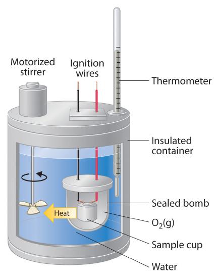
Constant-Volume Calorimetry: Enthalpies of Combustion

A bomb calorimeter is a an instrument that can be used to measure the enthalpies of reaction constant for combustion reactions, the enthalpy of combustion. Although we will not be doing bomb calorimeter calculations in this class, the concept is easily understood. You place a mass of a combustible material in the calorimeter, fill the bomb with high pressure oxygen and ignite it. You then measure the temperature, and calculate the enthalpy of combustion. This can then be repeated for a variety of combustible substances, and you can tabulate a thermodynamic table of combustion enthalpies.

In the next section we will use combustion enthalpies in multiple problems, and the reason they are being mentioned is so you can understand where the data comes from.

 

Contributors

• Robert Belford (UA of Little Rock)
• Ronia Kattoum (UA of Little Rock)