
4.7 Stoichiometry of Reactions in Aqueous Solutions
- Page ID
- 158429
\( \newcommand{\vecs}[1]{\overset { \scriptstyle \rightharpoonup} {\mathbf{#1}} } \)
\( \newcommand{\vecd}[1]{\overset{-\!-\!\rightharpoonup}{\vphantom{a}\smash {#1}}} \)
\( \newcommand{\id}{\mathrm{id}}\) \( \newcommand{\Span}{\mathrm{span}}\)
( \newcommand{\kernel}{\mathrm{null}\,}\) \( \newcommand{\range}{\mathrm{range}\,}\)
\( \newcommand{\RealPart}{\mathrm{Re}}\) \( \newcommand{\ImaginaryPart}{\mathrm{Im}}\)
\( \newcommand{\Argument}{\mathrm{Arg}}\) \( \newcommand{\norm}[1]{\| #1 \|}\)
\( \newcommand{\inner}[2]{\langle #1, #2 \rangle}\)
\( \newcommand{\Span}{\mathrm{span}}\)
\( \newcommand{\id}{\mathrm{id}}\)
\( \newcommand{\Span}{\mathrm{span}}\)
\( \newcommand{\kernel}{\mathrm{null}\,}\)
\( \newcommand{\range}{\mathrm{range}\,}\)
\( \newcommand{\RealPart}{\mathrm{Re}}\)
\( \newcommand{\ImaginaryPart}{\mathrm{Im}}\)
\( \newcommand{\Argument}{\mathrm{Arg}}\)
\( \newcommand{\norm}[1]{\| #1 \|}\)
\( \newcommand{\inner}[2]{\langle #1, #2 \rangle}\)
\( \newcommand{\Span}{\mathrm{span}}\) \( \newcommand{\AA}{\unicode[.8,0]{x212B}}\)
\( \newcommand{\vectorA}[1]{\vec{#1}} % arrow\)
\( \newcommand{\vectorAt}[1]{\vec{\text{#1}}} % arrow\)
\( \newcommand{\vectorB}[1]{\overset { \scriptstyle \rightharpoonup} {\mathbf{#1}} } \)
\( \newcommand{\vectorC}[1]{\textbf{#1}} \)
\( \newcommand{\vectorD}[1]{\overrightarrow{#1}} \)
\( \newcommand{\vectorDt}[1]{\overrightarrow{\text{#1}}} \)
\( \newcommand{\vectE}[1]{\overset{-\!-\!\rightharpoonup}{\vphantom{a}\smash{\mathbf {#1}}}} \)
\( \newcommand{\vecs}[1]{\overset { \scriptstyle \rightharpoonup} {\mathbf{#1}} } \)
\( \newcommand{\vecd}[1]{\overset{-\!-\!\rightharpoonup}{\vphantom{a}\smash {#1}}} \)
\(\newcommand{\avec}{\mathbf a}\) \(\newcommand{\bvec}{\mathbf b}\) \(\newcommand{\cvec}{\mathbf c}\) \(\newcommand{\dvec}{\mathbf d}\) \(\newcommand{\dtil}{\widetilde{\mathbf d}}\) \(\newcommand{\evec}{\mathbf e}\) \(\newcommand{\fvec}{\mathbf f}\) \(\newcommand{\nvec}{\mathbf n}\) \(\newcommand{\pvec}{\mathbf p}\) \(\newcommand{\qvec}{\mathbf q}\) \(\newcommand{\svec}{\mathbf s}\) \(\newcommand{\tvec}{\mathbf t}\) \(\newcommand{\uvec}{\mathbf u}\) \(\newcommand{\vvec}{\mathbf v}\) \(\newcommand{\wvec}{\mathbf w}\) \(\newcommand{\xvec}{\mathbf x}\) \(\newcommand{\yvec}{\mathbf y}\) \(\newcommand{\zvec}{\mathbf z}\) \(\newcommand{\rvec}{\mathbf r}\) \(\newcommand{\mvec}{\mathbf m}\) \(\newcommand{\zerovec}{\mathbf 0}\) \(\newcommand{\onevec}{\mathbf 1}\) \(\newcommand{\real}{\mathbb R}\) \(\newcommand{\twovec}[2]{\left[\begin{array}{r}#1 \\ #2 \end{array}\right]}\) \(\newcommand{\ctwovec}[2]{\left[\begin{array}{c}#1 \\ #2 \end{array}\right]}\) \(\newcommand{\threevec}[3]{\left[\begin{array}{r}#1 \\ #2 \\ #3 \end{array}\right]}\) \(\newcommand{\cthreevec}[3]{\left[\begin{array}{c}#1 \\ #2 \\ #3 \end{array}\right]}\) \(\newcommand{\fourvec}[4]{\left[\begin{array}{r}#1 \\ #2 \\ #3 \\ #4 \end{array}\right]}\) \(\newcommand{\cfourvec}[4]{\left[\begin{array}{c}#1 \\ #2 \\ #3 \\ #4 \end{array}\right]}\) \(\newcommand{\fivevec}[5]{\left[\begin{array}{r}#1 \\ #2 \\ #3 \\ #4 \\ #5 \\ \end{array}\right]}\) \(\newcommand{\cfivevec}[5]{\left[\begin{array}{c}#1 \\ #2 \\ #3 \\ #4 \\ #5 \\ \end{array}\right]}\) \(\newcommand{\mattwo}[4]{\left[\begin{array}{rr}#1 \amp #2 \\ #3 \amp #4 \\ \end{array}\right]}\) \(\newcommand{\laspan}[1]{\text{Span}\{#1\}}\) \(\newcommand{\bcal}{\cal B}\) \(\newcommand{\ccal}{\cal C}\) \(\newcommand{\scal}{\cal S}\) \(\newcommand{\wcal}{\cal W}\) \(\newcommand{\ecal}{\cal E}\) \(\newcommand{\coords}[2]{\left\{#1\right\}_{#2}}\) \(\newcommand{\gray}[1]{\color{gray}{#1}}\) \(\newcommand{\lgray}[1]{\color{lightgray}{#1}}\) \(\newcommand{\rank}{\operatorname{rank}}\) \(\newcommand{\row}{\text{Row}}\) \(\newcommand{\col}{\text{Col}}\) \(\renewcommand{\row}{\text{Row}}\) \(\newcommand{\nul}{\text{Nul}}\) \(\newcommand{\var}{\text{Var}}\) \(\newcommand{\corr}{\text{corr}}\) \(\newcommand{\len}[1]{\left|#1\right|}\) \(\newcommand{\bbar}{\overline{\bvec}}\) \(\newcommand{\bhat}{\widehat{\bvec}}\) \(\newcommand{\bperp}{\bvec^\perp}\) \(\newcommand{\xhat}{\widehat{\xvec}}\) \(\newcommand{\vhat}{\widehat{\vvec}}\) \(\newcommand{\uhat}{\widehat{\uvec}}\) \(\newcommand{\what}{\widehat{\wvec}}\) \(\newcommand{\Sighat}{\widehat{\Sigma}}\) \(\newcommand{\lt}{<}\) \(\newcommand{\gt}{>}\) \(\newcommand{\amp}{&}\) \(\definecolor{fillinmathshade}{gray}{0.9}\)Learning Objectives
- Apply stoichiometric calculations to reactions in solution
- Determine limiting reagents, excess reagents, theoretical yield for reactions in solution
Stoichiometry in Solutions
At the beginning of this chapter we covered stoichiometry of reactions where everything was a solid, and we used the mass and formula weight to calculate the moles of reactants or products consumed or produced.
The following pathway should be familiar for such calculations:
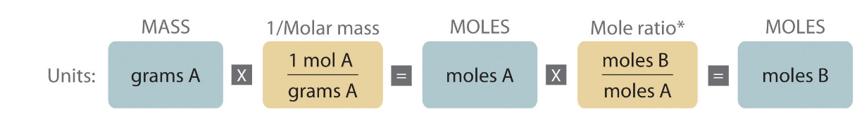
Figure 4.7.1 Source: Chapter 12.2: Stoichiometry of Reactions in Solution
However, for a reaction to proceed, reactants must come into contact with each other. One way of enabling this mobility is to dissolve the reactants into a solvent creating a solution. Unless you have a pure substance, you can not use mass to measure the number of particles, as you are weighing both the solvent and solute(s). So if you have a solution, you need to know the concentration, and the most common way of representing chemical concentrations is the molarity. The following possible pathways for stroichiometric conversions.

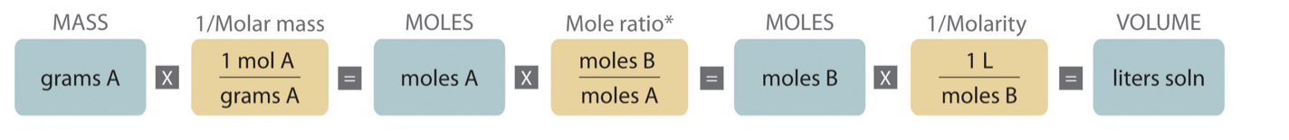
Figure 4.7.2: The top solution map is used when you have the volume of a solution with a given concentration and you are asked to solve for the mass of a solid produced or reacted. The bottom solution map is used if you start with the mass of the solid and you are trying to find the volume of the solution that is reacted or produced.
Source: Chapter 12.2: Stoichiometry of Reactions in Solution
Example \(\PageIndex{1}\)
What volume of 1.25 M HCl solution is required to fully react with 2.5440 grams of magnesium metal?
Solution
Given: concentration of HCl = 1.25 M (1.25 moles HCl/1 L of solution), mass of Mg = 2.5440 gram
Strategy:
1. Write the balanced molecular equation.
2. Create a solution map
3. Solve
Solution:
1. Mg(s) + 2 HCl(aq) → MgCl2(aq) + H2(g)
2. Mass of Mg → Moles of Mg → Moles of HCl → Volume of HCl solution
3. Set up using dimensional analysis:

Recap: It look like we would need 167 mL of 1.25 M HCl solution to fully react the 2.5440 g of Mg.
Exercise \(\PageIndex{1}\)
Sodium bicarbonate (baking soda) is often used in chemistry laboratories to neutralize acid spills. Suppose that you spilled 250.0 mL of 2.50 M sulfuric acid solution, what mass of sodium bicarbonate to yo need to neutralize it?
- Answer
-
Balanced Molecular Equation: 2 NaHCO3(s) + H2SO4(aq) → Na2SO4(aq) + 2 H2O(l) + 2 CO2(g)
Solution Map: volume of H2SO4 solution (mL) → L of H2SO4 solution→ moles of H2SO4 → moles NaHCO3 → mass of NaHCO3
Solve:

So, need 105 grams of baking soda to neutralize the 250.0 mL of 2.50 M sulfuric acid that was spilled.
Limiting Reagents in Solutions
We have seen how we can determine the limiting reagent, excess reagent, and theoretical yield when we started with the mass of two reactants. However, practically speaking, many of those reactants are in solutions in the laboratory. We can still determine the limiting reagent, excess reagent, and theoretical yield for reactants even when they are in solution. Let's take a look at an example of how we would approach such a problem.
Example \(\PageIndex{2}\)
You dissolve 10.0 grams of copper(II) sulfate in 500. mL of 0.100 M sodium phosphate.
1. Write the balanced molecular equation for the reaction that takes place.
2. Identify the limiting reagent, the excess reagent, and calculate the theoretical yield of the precipitate produced.
3. Determine the concentration of excess reagent
4. Determine the concentration of spectator ions
Solution
1. Write the balanced molecular equation for the reaction that takes place.
2. Identify the limiting reagent, the excess reagent, and calculate the theoretical yield of the precipitate produced.
Fast Method:
Fast Method Explained: Show the steps of the fast method
3. Determine the concentration of excess reagent
4. Determine the concentration of spectator ions
Note: You must have a balanced chemical reaction in order to solve stoichiometry problems correctly.
Contributors
- Robert Belford (UA of Little Rock)
- Ronia Kattoum (UA of Little Rock)