4.8 Stoichiometry of Reactions in Solution - Titrations

Titrations

In section 4.4 we introduced the analytical quantitative analysis technique of titrations that can be used to identify the quantity of an unknown. We will look at two types of titrations; acid/base titrations and Redox titrations. In both of these you have your unknown, that analyte, and a known, the titrant. You then add the titrant to the analyte until they are in stoichiometric proportions, and then by using the relationships of the balanced equation you can determine the quantity of the unknown.

General technique of a titration.

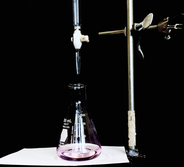
In a titration you place the analyte of unknown concentration into an Erylenmeyer flask (or similar container), and then use a burette to add the standard to the unknown, and measure the quantity of standard required to completely react with the analyte. Initially, the analyte is the excess reagent, at the equivalence point you have added just enough of the standard to react with all of the analyte, and after the equivalence point there is excess standard. So the objective is to be able to identify how much of the standard can be added so that they are in stoichiometric proportions. If the products have a different color than the reactants, you can use the color change to indicate when they are in stoichomtric proportions. If not, you can add an indicator that changes color when all of the analyte has been used.

Acid-Base Titrations

These are a technique for determining the concentration of unknown acids or bases. In the case of an acid, you determine the volume of a strong base requried to neutralize it, and then use the stoichiometery of the neutralization equation to determine the moles acid initially present, and then divide by the inital volume of the acid to determine it's concentration. In the case of an unknown base, you titrate with an acid of known concentration.

Example: A chemist needs to know the concentration of a 50 gallon drum of sulfuric acid. So the chemist uses a 25 mL volumetric pipette to transfer 25.00 mL of the unknown acid and to an Erlenmeyer Flask and adds 2 drops in an indicator that changes color when the acid is neutralized. This solution is then titrated with 0.100M sodium hydroxide and it takes 30.00 mL to neutralize the 25.00 mL of sulfuric acid.

Step 1: Write down the balanced equation and under each entity write what is given in the problem statement.

H₂SO₄(aq) + 2NaOH(aq) --> Na₂SO₄(aq) + 2H₂O(l)
M =? M = 0.100 M
V= 25.00mL V= 30.00 mL

Step 2: Calculate moles acid (n_A) present when from the amount of base required to neutralize it. Note, from the equation, it takes two moles of sodium hydroxide to neurtalize one mole of sufluric acid.

\[n_{a}=\left ( 0.100M\: Na)H \right )\left ( 0.03000L \right )\left ( \frac{molH_{2}SO_{4}}{2\, mol\: NaOH} \right )=0.00150\: mol\, H_{2}SO_{4}\]

Step 3: Divide by the volume of acid titrated, and this gives the concentration of the acid in the 50 gallon drum

0.00150/0.02500 = 0.0600L = 60.0 mL

 

Acid/Base titration video

The ideal gas law is easy to remember and apply in solving problems, as long as you get the proper values a

Redox Titration

These are electron transfer reactions and use the stoichiometery fo the balanced equation to determine the concentration of an unknown.

 

Redox Titration Video

What is the Fe⁺² concentration of a solution if 25.00 mL of the solution requires 30.24 mL of 0.0300 M potassium permangante to titrate the iron.

The balanced net ionic equation is,

MnO₄^- (aq) + 5 Fe⁺² + 8H₃O⁺(aq) --> Mn⁺²(aq) + 5Fe⁺³(aq) + 12H₂O(l)