
8.6: Molecular Geometries
- Page ID
- 52692

\( \newcommand{\vecs}[1]{\overset { \scriptstyle \rightharpoonup} {\mathbf{#1}} } \)
\( \newcommand{\vecd}[1]{\overset{-\!-\!\rightharpoonup}{\vphantom{a}\smash {#1}}} \)
\( \newcommand{\id}{\mathrm{id}}\) \( \newcommand{\Span}{\mathrm{span}}\)
( \newcommand{\kernel}{\mathrm{null}\,}\) \( \newcommand{\range}{\mathrm{range}\,}\)
\( \newcommand{\RealPart}{\mathrm{Re}}\) \( \newcommand{\ImaginaryPart}{\mathrm{Im}}\)
\( \newcommand{\Argument}{\mathrm{Arg}}\) \( \newcommand{\norm}[1]{\| #1 \|}\)
\( \newcommand{\inner}[2]{\langle #1, #2 \rangle}\)
\( \newcommand{\Span}{\mathrm{span}}\)
\( \newcommand{\id}{\mathrm{id}}\)
\( \newcommand{\Span}{\mathrm{span}}\)
\( \newcommand{\kernel}{\mathrm{null}\,}\)
\( \newcommand{\range}{\mathrm{range}\,}\)
\( \newcommand{\RealPart}{\mathrm{Re}}\)
\( \newcommand{\ImaginaryPart}{\mathrm{Im}}\)
\( \newcommand{\Argument}{\mathrm{Arg}}\)
\( \newcommand{\norm}[1]{\| #1 \|}\)
\( \newcommand{\inner}[2]{\langle #1, #2 \rangle}\)
\( \newcommand{\Span}{\mathrm{span}}\) \( \newcommand{\AA}{\unicode[.8,0]{x212B}}\)
\( \newcommand{\vectorA}[1]{\vec{#1}} % arrow\)
\( \newcommand{\vectorAt}[1]{\vec{\text{#1}}} % arrow\)
\( \newcommand{\vectorB}[1]{\overset { \scriptstyle \rightharpoonup} {\mathbf{#1}} } \)
\( \newcommand{\vectorC}[1]{\textbf{#1}} \)
\( \newcommand{\vectorD}[1]{\overrightarrow{#1}} \)
\( \newcommand{\vectorDt}[1]{\overrightarrow{\text{#1}}} \)
\( \newcommand{\vectE}[1]{\overset{-\!-\!\rightharpoonup}{\vphantom{a}\smash{\mathbf {#1}}}} \)
\( \newcommand{\vecs}[1]{\overset { \scriptstyle \rightharpoonup} {\mathbf{#1}} } \)
\( \newcommand{\vecd}[1]{\overset{-\!-\!\rightharpoonup}{\vphantom{a}\smash {#1}}} \)
\(\newcommand{\avec}{\mathbf a}\) \(\newcommand{\bvec}{\mathbf b}\) \(\newcommand{\cvec}{\mathbf c}\) \(\newcommand{\dvec}{\mathbf d}\) \(\newcommand{\dtil}{\widetilde{\mathbf d}}\) \(\newcommand{\evec}{\mathbf e}\) \(\newcommand{\fvec}{\mathbf f}\) \(\newcommand{\nvec}{\mathbf n}\) \(\newcommand{\pvec}{\mathbf p}\) \(\newcommand{\qvec}{\mathbf q}\) \(\newcommand{\svec}{\mathbf s}\) \(\newcommand{\tvec}{\mathbf t}\) \(\newcommand{\uvec}{\mathbf u}\) \(\newcommand{\vvec}{\mathbf v}\) \(\newcommand{\wvec}{\mathbf w}\) \(\newcommand{\xvec}{\mathbf x}\) \(\newcommand{\yvec}{\mathbf y}\) \(\newcommand{\zvec}{\mathbf z}\) \(\newcommand{\rvec}{\mathbf r}\) \(\newcommand{\mvec}{\mathbf m}\) \(\newcommand{\zerovec}{\mathbf 0}\) \(\newcommand{\onevec}{\mathbf 1}\) \(\newcommand{\real}{\mathbb R}\) \(\newcommand{\twovec}[2]{\left[\begin{array}{r}#1 \\ #2 \end{array}\right]}\) \(\newcommand{\ctwovec}[2]{\left[\begin{array}{c}#1 \\ #2 \end{array}\right]}\) \(\newcommand{\threevec}[3]{\left[\begin{array}{r}#1 \\ #2 \\ #3 \end{array}\right]}\) \(\newcommand{\cthreevec}[3]{\left[\begin{array}{c}#1 \\ #2 \\ #3 \end{array}\right]}\) \(\newcommand{\fourvec}[4]{\left[\begin{array}{r}#1 \\ #2 \\ #3 \\ #4 \end{array}\right]}\) \(\newcommand{\cfourvec}[4]{\left[\begin{array}{c}#1 \\ #2 \\ #3 \\ #4 \end{array}\right]}\) \(\newcommand{\fivevec}[5]{\left[\begin{array}{r}#1 \\ #2 \\ #3 \\ #4 \\ #5 \\ \end{array}\right]}\) \(\newcommand{\cfivevec}[5]{\left[\begin{array}{c}#1 \\ #2 \\ #3 \\ #4 \\ #5 \\ \end{array}\right]}\) \(\newcommand{\mattwo}[4]{\left[\begin{array}{rr}#1 \amp #2 \\ #3 \amp #4 \\ \end{array}\right]}\) \(\newcommand{\laspan}[1]{\text{Span}\{#1\}}\) \(\newcommand{\bcal}{\cal B}\) \(\newcommand{\ccal}{\cal C}\) \(\newcommand{\scal}{\cal S}\) \(\newcommand{\wcal}{\cal W}\) \(\newcommand{\ecal}{\cal E}\) \(\newcommand{\coords}[2]{\left\{#1\right\}_{#2}}\) \(\newcommand{\gray}[1]{\color{gray}{#1}}\) \(\newcommand{\lgray}[1]{\color{lightgray}{#1}}\) \(\newcommand{\rank}{\operatorname{rank}}\) \(\newcommand{\row}{\text{Row}}\) \(\newcommand{\col}{\text{Col}}\) \(\renewcommand{\row}{\text{Row}}\) \(\newcommand{\nul}{\text{Nul}}\) \(\newcommand{\var}{\text{Var}}\) \(\newcommand{\corr}{\text{corr}}\) \(\newcommand{\len}[1]{\left|#1\right|}\) \(\newcommand{\bbar}{\overline{\bvec}}\) \(\newcommand{\bhat}{\widehat{\bvec}}\) \(\newcommand{\bperp}{\bvec^\perp}\) \(\newcommand{\xhat}{\widehat{\xvec}}\) \(\newcommand{\vhat}{\widehat{\vvec}}\) \(\newcommand{\uhat}{\widehat{\uvec}}\) \(\newcommand{\what}{\widehat{\wvec}}\) \(\newcommand{\Sighat}{\widehat{\Sigma}}\) \(\newcommand{\lt}{<}\) \(\newcommand{\gt}{>}\) \(\newcommand{\amp}{&}\) \(\definecolor{fillinmathshade}{gray}{0.9}\)Introduction
There is a three step approach to determining the geometry of a molecule.
- Determine the Lewis dot structure of the compound.
- Determine the Electron geometry from the Lewis dot structure.
- Determine the molecular geometry.
It is very important from the onset that students understand the difference between electronic geometry and molecular geometry. In calculating electronic geometry we use the Valence Shell Electron Pair Repulsion (VSEPR) model, which states that the lowest geometry for electronic orbitals around a positive nucleus is for the orbitals to be as far away as possible. Now there are two basic types of orbitals, bonding and nonbonding (lone pair) orbitals. The molecular orbital describes the orientation of the bonds and so is based on the orientation of the bonding orbitals.
VSPER
VSEPR (Valence Shell Electron Repulsion Theory) is used to determine the geometry of the orbitals around a nucleus. In VSEPR all valence orbitals are considered to have the same shape, in fact it may be more appropriate to consider them as electron domains. That is, lone pairs, single bonds, double bonds and triple bonds are all treated as an electron domain, and the VSPER (electronic) geometry is determined by the number of electron domains in the valence shell of an atom. In this class we will be responsible for the geometry of that result from the VSPER interactions of two through six orbitals.
Video \(\PageIndex{1}\) is a very short video showing the five VSPER electronic geometries for atoms with between 2 and 6 electron domains, the steric number. In watching video \(\PageIndex{1}\) you should note how the geometry changes as the steric number changes and additional orbitals are successively added to the central atom. The five geometries are summarized in table \(\PageIndex{1}\).
The five VSEPR geometries are summarized in table \(\PageIndex{1}\).
| # Electron Domains (Steric Number) |
VSEPR Geometry | Angle Between Electron Domains | |
|---|---|---|---|
| 2 | linear | 180o |  |
| 3 | trigonal planar | 120o | 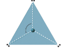 |
| 4 | tetrahedral | 109.5o |  |
| 5 | trigonal bipyramidal | 90o, 120o | 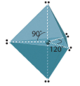 |
| 6 | octahedral | 90o | 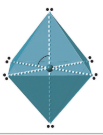 |
Molecular Geometry
After calculating the electronic geometry from VESPR we can determine the molecular geometry based on the bonding orbitals. If there are no lone pairs and all orbitals are bonding, then the molecular geometry is the electronic geometry. Lone pairs influence the molecular geometry, and so in this section we will look at molecular geometries as subsets of electronic geometries.
Before proceeding, please watch the follow YouTube
Figure \(\PageIndex{1}\) shows the various molecular geometries for the five VESPR electronic geometries with 2 to 6 electron domains. When there are no lone pairs the molecular geometry is the electron (VESPR) geometry. When there are lone pairs, you need to look at the structure and recognize the names and bond angles. Note, this work ignores the trivial geometry of two atoms like HCl or H2, as they must be linear, but when you have three atoms, they can be linear or bent.
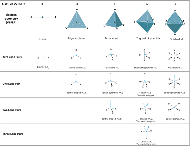
Figure \(\PageIndex{1}\): Overview of molecular geometries based on bonding orbitals of VSEPR electronic structures.
Two Electron Domains
Three atoms result in two electron domains and the structure is linear. There are three common types of molecules that form these structures, molecules with two single bonds (BeH2), molecules with a two double bonds (CO2) and molecules with a single and triple bond (HCN).
| H-Be-H | O=C=O | \(H-C\equiv N\) |
| BeH2 | CO2 | HCN |
Note, Beryllium can have less than an octet, while carbon can not. Also note that the double bond in carbon dioxide and the triple bond in hydrogen cyanide are both treated as a single electron domain
Three Electron Domains
There are two molecular geometries that can come out of three electron domains, trigonal planar (no lone pairs) and bent with \(\approx \)120° bond angle (one lone pair) .
0 lone pairs
These are of the form AX3, where X represents an atom that is bonded to three other atoms, and for which there are no lone pairs.
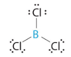 |
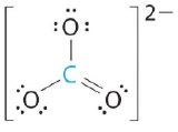 |
| BCl3 (Group IIIA can have less than an octet) | CO3-2 (note there are resonance structures for carbonate) |
1 lone pair
These are atoms of the form AX2E, where E represents a lone pair. Examples are SO2 and O3. Note, the lone pair takes up more space than the bonding pair, so the bond angle is less then the ideal 120o.

Four Electron Domains
All atoms with four electron domains have tetrahedral electronic geometry
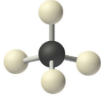
0 Lone Pairs
These are of the form AX4 and the molecular geometry is the same as the electronic geometry
1 Lone Pair
These are of the form AX3E and have trigonal pyramidal molecular geometries. Note the bond angle is less than the ideal because the lone pair take up more space

2 Lone Pairs
These are of the form AX2E2 and have bent angles, which in the case of water are 104.5oC
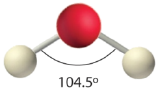
These are of the form AX2E2 and have bent angles, which in the case of water are 104.5oC
Note
There are two bent geometries based on trigonal planar electronic geometry with one lone pair as exemplified by sulfur dioxide that has a bond angle a bit less than 120oC, and by tetrahedral electronic geometry with two lone pairs, as exemplified by water with 104.5oC bond angle.
Five Electron Domains
All molecules with 5 electron domains have trigonal bipyramidial electronic geometry. The central atom of these molecules must be in the third or higher period of the periodic table.

In Figure \(\PageIndex{7}\) you note that the two axial positions are linear to each other and if we define this axis as the z axis of the cartesian coordinate system, then the equatorial positions have a trigonal planar geometry in the xy plane. So the trigonal bipyramidal geometry is a superposition of linear and trigonal planar geometries. It is important to note that the bond angle between equatorial and axial positions (90o) is different than between two equatorial positions (120o).
0 Lone Pairs
As in the above cases, if there are no lone pairs, the electronic geometry is the molecular geometry.

1 Lone Pair
These are of the form AX4E and have a "See-Saw" geometry, which is also classified as a distorted tetrahedron. Sulfur tetrafluoride ( SF4) has such a structure.
Note
The Lone pair can take two positions, axial or equatorial. The lone pair goes into the equatorial position because it takes up more space, and there is more room in the equatorial positions. This can be seen from Figure \(\PageIndex{7}\), where it is clear that the 90o bonds bring the atoms closer than the 120o bonds, and each axial position has three 90o bond interactions while each equatorial has two (and two 120o) bond interactions. As the lone pairs take up more space, they move into the equatorial positions.

2 Lone Pairs
These are of the form of AX3E2 have trigonal bipyramidal electronic geometry and "T-shaped" molecular geometry. Bromine triflouride (BrF3) is an example of a molecule with 5 electron domains and two lone pairs (Figure .

Figure \(\PageIndex{10}\): Lewis dot diagram of bromine trifluoride showing two lone pairs.
There are three ways of distributing the lone pairs between the axial and equatorial positions and the lone pairs always go on the equatorial positions because these are the least confined. This can be seen in Figure \(\PageIndex{11}\)

Once again, the lone pairs go into the equatorial positions.
3 Lone Pairs
These are of the form AX2E3 and and the trigonal bipyramidal electronic structure results in a linear molecular structure. Triiodide (I3−) is an example of this geometry.

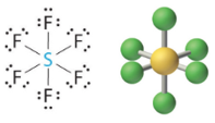
Six Electron Domains
Six electron domains form an octahedron, a polyhedron with 8 faces, but the electron pair geometry has linear orientations along the 3 Cartesian coordinate axis. Therefore the octahedral represents 6 electron domains along the Cartesian axis (Figure \(\PageIndex{13}\)).
 Figure \(\PageIndex{13}\): Six domains has electron pairs oriented along the 3 Cartesian coordinate axes
0 Lone Pairs
1 Lone Pair

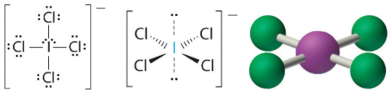
2 Lone Pairs
These structures are of the form AX4E2and form square planar structures. Iodine tetrachloride ion (ICl4−). T
Molecules with No Single Central Atom
The VSEPR model can be used to predict the structure of somewhat more complex molecules with no single central atom by treating them as linked AXmEn fragments. We will demonstrate with methyl isocyanate (CH3–N=C=O), a volatile and highly toxic molecule that is used to produce the pesticide Sevin. In 1984, large quantities of Sevin were accidentally released in Bhopal, India, when water leaked into storage tanks. The resulting highly exothermic reaction caused a rapid increase in pressure that ruptured the tanks, releasing large amounts of methyl isocyanate that killed approximately 3800 people and wholly or partially disabled about 50,000 others. In addition, there was significant damage to livestock and crops.
We can treat methyl isocyanate (CH3–N=C=O), as linked AXmEn fragments beginning with the left carbon, followed by the nitrogen and then the second carbon
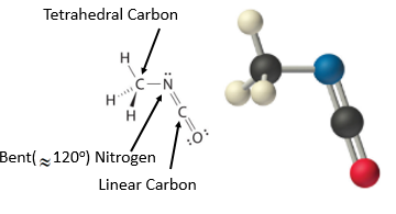
Figure \(\PageIndex{17}\): Geometric structure of methyl isocyanate (CH3–N=C=O), note there is no rotation around the double bonds only the single CN bond can rotate.
Contributors and Attributions
Robert E. Belford (University of Arkansas Little Rock; Department of Chemistry). The breadth, depth and veracity of this work is the responsibility of Robert E. Belford, rebelford@ualr.edu. You should contact him if you have any concerns. This material has both original contributions, and content built upon prior contributions of the LibreTexts Community and other resources, including but not limited to:
- Anonymous
- Modifications of material modified by Joshua Halpern, Scott Sinex and Scott Johnson