
6.5: The Modern View of Electronic Structure
- Page ID
- 52800

\( \newcommand{\vecs}[1]{\overset { \scriptstyle \rightharpoonup} {\mathbf{#1}} } \)
\( \newcommand{\vecd}[1]{\overset{-\!-\!\rightharpoonup}{\vphantom{a}\smash {#1}}} \)
\( \newcommand{\id}{\mathrm{id}}\) \( \newcommand{\Span}{\mathrm{span}}\)
( \newcommand{\kernel}{\mathrm{null}\,}\) \( \newcommand{\range}{\mathrm{range}\,}\)
\( \newcommand{\RealPart}{\mathrm{Re}}\) \( \newcommand{\ImaginaryPart}{\mathrm{Im}}\)
\( \newcommand{\Argument}{\mathrm{Arg}}\) \( \newcommand{\norm}[1]{\| #1 \|}\)
\( \newcommand{\inner}[2]{\langle #1, #2 \rangle}\)
\( \newcommand{\Span}{\mathrm{span}}\)
\( \newcommand{\id}{\mathrm{id}}\)
\( \newcommand{\Span}{\mathrm{span}}\)
\( \newcommand{\kernel}{\mathrm{null}\,}\)
\( \newcommand{\range}{\mathrm{range}\,}\)
\( \newcommand{\RealPart}{\mathrm{Re}}\)
\( \newcommand{\ImaginaryPart}{\mathrm{Im}}\)
\( \newcommand{\Argument}{\mathrm{Arg}}\)
\( \newcommand{\norm}[1]{\| #1 \|}\)
\( \newcommand{\inner}[2]{\langle #1, #2 \rangle}\)
\( \newcommand{\Span}{\mathrm{span}}\) \( \newcommand{\AA}{\unicode[.8,0]{x212B}}\)
\( \newcommand{\vectorA}[1]{\vec{#1}} % arrow\)
\( \newcommand{\vectorAt}[1]{\vec{\text{#1}}} % arrow\)
\( \newcommand{\vectorB}[1]{\overset { \scriptstyle \rightharpoonup} {\mathbf{#1}} } \)
\( \newcommand{\vectorC}[1]{\textbf{#1}} \)
\( \newcommand{\vectorD}[1]{\overrightarrow{#1}} \)
\( \newcommand{\vectorDt}[1]{\overrightarrow{\text{#1}}} \)
\( \newcommand{\vectE}[1]{\overset{-\!-\!\rightharpoonup}{\vphantom{a}\smash{\mathbf {#1}}}} \)
\( \newcommand{\vecs}[1]{\overset { \scriptstyle \rightharpoonup} {\mathbf{#1}} } \)
\( \newcommand{\vecd}[1]{\overset{-\!-\!\rightharpoonup}{\vphantom{a}\smash {#1}}} \)
\(\newcommand{\avec}{\mathbf a}\) \(\newcommand{\bvec}{\mathbf b}\) \(\newcommand{\cvec}{\mathbf c}\) \(\newcommand{\dvec}{\mathbf d}\) \(\newcommand{\dtil}{\widetilde{\mathbf d}}\) \(\newcommand{\evec}{\mathbf e}\) \(\newcommand{\fvec}{\mathbf f}\) \(\newcommand{\nvec}{\mathbf n}\) \(\newcommand{\pvec}{\mathbf p}\) \(\newcommand{\qvec}{\mathbf q}\) \(\newcommand{\svec}{\mathbf s}\) \(\newcommand{\tvec}{\mathbf t}\) \(\newcommand{\uvec}{\mathbf u}\) \(\newcommand{\vvec}{\mathbf v}\) \(\newcommand{\wvec}{\mathbf w}\) \(\newcommand{\xvec}{\mathbf x}\) \(\newcommand{\yvec}{\mathbf y}\) \(\newcommand{\zvec}{\mathbf z}\) \(\newcommand{\rvec}{\mathbf r}\) \(\newcommand{\mvec}{\mathbf m}\) \(\newcommand{\zerovec}{\mathbf 0}\) \(\newcommand{\onevec}{\mathbf 1}\) \(\newcommand{\real}{\mathbb R}\) \(\newcommand{\twovec}[2]{\left[\begin{array}{r}#1 \\ #2 \end{array}\right]}\) \(\newcommand{\ctwovec}[2]{\left[\begin{array}{c}#1 \\ #2 \end{array}\right]}\) \(\newcommand{\threevec}[3]{\left[\begin{array}{r}#1 \\ #2 \\ #3 \end{array}\right]}\) \(\newcommand{\cthreevec}[3]{\left[\begin{array}{c}#1 \\ #2 \\ #3 \end{array}\right]}\) \(\newcommand{\fourvec}[4]{\left[\begin{array}{r}#1 \\ #2 \\ #3 \\ #4 \end{array}\right]}\) \(\newcommand{\cfourvec}[4]{\left[\begin{array}{c}#1 \\ #2 \\ #3 \\ #4 \end{array}\right]}\) \(\newcommand{\fivevec}[5]{\left[\begin{array}{r}#1 \\ #2 \\ #3 \\ #4 \\ #5 \\ \end{array}\right]}\) \(\newcommand{\cfivevec}[5]{\left[\begin{array}{c}#1 \\ #2 \\ #3 \\ #4 \\ #5 \\ \end{array}\right]}\) \(\newcommand{\mattwo}[4]{\left[\begin{array}{rr}#1 \amp #2 \\ #3 \amp #4 \\ \end{array}\right]}\) \(\newcommand{\laspan}[1]{\text{Span}\{#1\}}\) \(\newcommand{\bcal}{\cal B}\) \(\newcommand{\ccal}{\cal C}\) \(\newcommand{\scal}{\cal S}\) \(\newcommand{\wcal}{\cal W}\) \(\newcommand{\ecal}{\cal E}\) \(\newcommand{\coords}[2]{\left\{#1\right\}_{#2}}\) \(\newcommand{\gray}[1]{\color{gray}{#1}}\) \(\newcommand{\lgray}[1]{\color{lightgray}{#1}}\) \(\newcommand{\rank}{\operatorname{rank}}\) \(\newcommand{\row}{\text{Row}}\) \(\newcommand{\col}{\text{Col}}\) \(\renewcommand{\row}{\text{Row}}\) \(\newcommand{\nul}{\text{Nul}}\) \(\newcommand{\var}{\text{Var}}\) \(\newcommand{\corr}{\text{corr}}\) \(\newcommand{\len}[1]{\left|#1\right|}\) \(\newcommand{\bbar}{\overline{\bvec}}\) \(\newcommand{\bhat}{\widehat{\bvec}}\) \(\newcommand{\bperp}{\bvec^\perp}\) \(\newcommand{\xhat}{\widehat{\xvec}}\) \(\newcommand{\vhat}{\widehat{\vvec}}\) \(\newcommand{\uhat}{\widehat{\uvec}}\) \(\newcommand{\what}{\widehat{\wvec}}\) \(\newcommand{\Sighat}{\widehat{\Sigma}}\) \(\newcommand{\lt}{<}\) \(\newcommand{\gt}{>}\) \(\newcommand{\amp}{&}\) \(\definecolor{fillinmathshade}{gray}{0.9}\)Schrödinger Wave Equation
The paradox described by Heisenberg’s uncertainty principle and the wavelike nature of subatomic particles such as the electron made it impossible to use the equations of classical physics to describe the motion of electrons in atoms. Scientists needed a new approach that took the wave behavior of the electron into account. In 1926, an Austrian physicist, Erwin Schrödinger (1887–1961; Nobel Prize in Physics, 1933), developed wave mechanics, a mathematical technique that describes the relationship between the motion of a particle that exhibits wavelike properties (such as an electron) and its allowed energies. This is a complex differential equation beyond the scope of this course that has the simplified form of
\[\hat{H}ψ=Eψ\]
Where \(\hat{H}\) is the Hamiltonian operator, which is a set of mathematical operations that work on the function \(\psi\) and can be used to determine the energy of the system. The Hamiltonian takes into account kinetic and potential energy interactions. When applied to the wave function solutions for spherical harmonics, which can be envisioned as standing waves of a fluid filled spherical object, the Schrödinger wave equation can be used to understand the different orbitals an electron can exist in a hydrogen-like atom (where one electron exists around a single nucleus).
Note
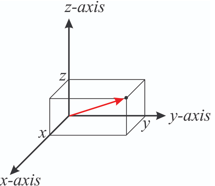
The wave function \(\psi\) for the hydrogen like atom can have very complex forms involving sinusoidal and exponential functions that can include imaginary numbers like \( \psi_{21\pm\ 1} = \dfrac {1}{\sqrt {64\pi}} \left(\dfrac {Z}{a_0}\right)^{\dfrac {3}{2}} \rho e^{-\rho/2} \sin(\theta) e^{\pm\ i\phi}\). These wave functions are typically described by two coordinate systems, the Cartesian (x,y,z) or spherical (r,\(\theta ,\phi\)).
 |
 |
| Cartesian Coordinates | Spherical coordinates |
Figure \(\PageIndex{1}\): The spherical coordinate system is easier than the Cartesian system to represent an electronic orbital. Note \(\theta\) varies from 0 to 360o while \(\phi\) varies from 0 to 180o.
Max Born set forth an interpretation of the square of these wave functions as probability density functions for the location of an electron, and we will define orbitals as regions in space where there is a 90% probability of finding an electron (as defined by the solutions to Schrödinger equation). It is important to distinguish the concept of orbita, which defines the location in space where one can find a tiny electron that shows wave-particle duality, in contrast to the orbit (of the Bohr) model that describes the location and trajectory of a macroscopic object like the moon in an orbit around a planet.
- Orbit - classical object in an orbit around another object, like the earth in an orbit around the sun. You can know both its position and momentum, that is, where it is and where it will be.
- Orbital - quantum object in an orbital where you have wave/particle duality and Heisenberg's uncertainty principle applies. You can not know both its position and momentum, and the orbital is a three dimensional probability function (\(\psi ^2\)), which in this class we loosely define as where the electron has a 90% probability of being.
In this class we will define each orbital by a unique set of quantum numbers.
Phet Simulation
The above simulation can help us review the various approaches we have taken so far.
Quantum Numbers
Schrödinger’s approach results in three quantum numbers that can be used to define an orbital (wave function), the principle (n), azimuthal (l), and magnetic (ml) quantum number. There is a fourth quantum number, the spin quantum number (ms) and electrons can reside in orbitals that are defined by these four quantum numbers. Every electron in an atom must reside in an orbital that contains a unique set of quantum numbers.
Principle Quantum Number (n)
The principal quantum number (n) tells the average relative distance of an electron from the nucleus:
\[n = 1, 2, 3, 4,… \]
As n increases for a given atom, so does the average distance of an electron from the nucleus. A negatively charged electron that is, on average, closer to the positively charged nucleus is attracted to the nucleus more strongly than an electron that is farther out in space. This means that electrons with higher values of n are easier to remove from an atom. All wavefunctions that have the same value of n are said to constitute a principal shell because those electrons have similar average distances from the nucleus. As you will see, the principal quantum number n corresponds to the n used by Bohr to describe electron orbits and by Rydberg to describe atomic energy levels. As we will see, these can also be related to the periods of the periodic table.
Azimuthal Quantum Number (l)
The second quantum number is often called the azimuthal quantum number (l). The value of l describes the shape of the region of space occupied by the electron. If you look at the standing waves in section 6.4.3.2 the value of l can be related to the number of nodes and so the first standing wave (n=1) has l=0 (there is no node).
The allowed values of l depend on the value of n and can range from 0 to n − 1:
\[l = 0, 1, 2,…, n − 1 \]
For example, if n = 1, l can be only 0; if n = 2, l can be 0 or 1; if n = 3, l can be 0,1, or 2; and so forth. For a given atom, all wavefunctions that have the same values of both n and l form a subshell. The regions of space occupied by electrons in the same subshell usually have the same shape, but they are oriented differently in space.
In naming orbitals we often denote the azmuthial number with a symbol. l=0 is an s orbital, l = 1 is a p orbital, l=2 is a d orbital and l=3 is an f orbital.
Magnetic Quantum Number (ml)
The third quantum number is the magnetic quantum number (\(m_l\)). The value of \(m_l\) describes the orientation of the region in space occupied by an electron with respect to an applied magnetic field.
For each value of n there are 2l+1 values of ml
The allowed values of \(m_l\) depend on the value of l: ml can range from −l to l in integral steps:
\[m_l = −l, −l + 1,…, 0,…, l − 1, l \]
For example, if \(l = 0\), \(m_l\) can be only 0; if l = 1, ml can be −1, 0, or +1; and if l = 2, ml can be −2, −1, 0, +1, or +2.
Each wavefunction with an allowed combination of n, l, and ml values describes an atomic orbital, a particular spatial distribution for an electron. For a given set of quantum numbers, each principal shell has a fixed number of subshells, and each subshell has a fixed number of orbitals.
Spin Quantum Number
There is a fourth quantum number, which is the electron spin quantum number. The above three quantum numbers come from the solutions of the Schrödinger wave equation and describe the distance from the nucleus, the shape and orientation of the electronic orbitals that can exist for a hydrogen like atom. But there are actually two orbitals within each of these orbitals, and these result from the intrinsic spin of an electrons, which produces an intrinsic magnetic field. this will be covered in section 6.7 of this Chapter and is being mentioned now so that students realize up front, that there are really four quantum numbers that define the electronic orbitals of an atom.
It should be noted that in 1928 Paul Dirac developed a relativistic wave equation, the Dirac Equation, that was consistent with both quantum mechanics and the theory of special relativity, and not only accounted for all four quantum numbers, but even introduced the concept of antimatter. We will hold off on dealing with the spin quantum number until section 6.7.
Naming Orbitals
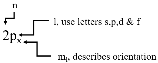
The first three quantum numbers define the geometric shapes of the orbitals and can be used to name them. The convention is to first indicate the principle quantum number (n), followed by a letter designating the azimuthal quantum number and then using a subscript to indicate the magnetic quantum number. The magnetic quantum number is often not specified. Note, the ml value may be the true values (-3,-2,-1,0,+1,+2,+3), or as we will see in the next section, expressions within the x,y,z Cartesian coordinate system.
 |
s: l=0 |
Number of Each Orbital
For each shell there are n orbitals. The following table shows the allowed orbitals for ground state configurations, for each shell (principle quantum number) you add an azimuthal orbital (the allowed values of l for each n are 0 to n-1), where l=0 is an s orbital, l=1 is a p, l=2 is a d....)
1s
2s, 2p
3s, 3p, 3d
4s, 4p, 4d, 4f
5s, 5p, 5d, 5f, 5g
6s, 6p, 6d, 6f, 6g, 6h
7s, 7p, 7d, 7f, 7g, 7h, 7i
As we shall see in the next Chapter, the structure of the periodic table is based on the filling of the orbitals in their lowest energy state, and the orbitals in orange (5g, 6g,6h,...) are of such high energy that electrons do not occupy them if the electron is in a ground state configuration.
Now because the are 2l+1 magnetic quantum numbers for each n, there are n2 potential orbitals for each principle quantum number
n= 1 as one s orbital = (1 total)
n=2 has one s and three p (4 total)
n=3 has one s, three p and 5 d (9 total)
n=4 has one s, three p, 5 d and 7 f (16 total)
....
| n | l | Subshell Designation | ml | Number of Orbitals in Subshell | Number of Orbitals in Shell |
|---|---|---|---|---|---|
| 1 | 0 | 1s | 0 | 1 | 1 |
| 2 | 0 | 2s | 0 | 1 | 4 |
| 1 | 2p | −1, 0, 1 | 3 | ||
| 3 | 0 | 3s | 0 | 1 | 9 |
| 1 | 3p | −1, 0, 1 | 3 | ||
| 2 | 3d | −2, −1, 0, 1, 2 | 5 | ||
| 4 | 0 | 4s | 0 | 1 | 16 |
| 1 | 4p | −1, 0, 1 | 3 | ||
| 2 | 4d | −2, −1, 0, 1, 2 | 5 | ||
| 3 | 4f | −3, −2, −1, 0, 1, 2, 3 | 7 |
Example\(\PageIndex{1}\): n=4 Shell Structure
How many subshells and orbitals are contained within the principal shell with n = 4?
Given: value of n
Asked for: number of subshells and orbitals in the principal shell
Strategy:
- Given n = 4, calculate the allowed values of l. From these allowed values, count the number of subshells.
- For each allowed value of l, calculate the allowed values of ml. The sum of the number of orbitals in each subshell is the number of orbitals in the principal shell.
Solution:
A We know that l can have all integral values from 0 to n − 1. If n = 4, then l can equal 0, 1, 2, or 3. Because the shell has four values of l, it has four subshells, each of which will contain a different number of orbitals, depending on the allowed values of ml.
B For l = 0, ml can be only 0, and thus the l = 0 subshell has only one orbital. For l = 1, ml can be 0 or ±1; thus the l = 1 subshell has three orbitals. For l = 2, ml can be 0, ±1, or ±2, so there are five orbitals in the l = 2 subshell. The last allowed value of l is l = 3, for which ml can be 0, ±1, ±2, or ±3, resulting in seven orbitals in the l = 3 subshell. The total number of orbitals in the n = 4 principal shell is the sum of the number of orbitals in each subshell and is equal to n2:
Exercise \(\PageIndex{1}\)
How many subshells and orbitals are in the principal shell with n = 3?
- Answer
-
3 subshells (s,p,d) and 9 orbitals (1 for l=0, 3 in p where l=1 and ml = -1, 0 and +1, and 5 for l=2 with ml = -2, -1, 0, +1 and +2)
Contributors and Attributions
Robert E. Belford (University of Arkansas Little Rock; Department of Chemistry). The breadth, depth and veracity of this work is the responsibility of Robert E. Belford, rebelford@ualr.edu. You should contact him if you have any concerns. This material has both original contributions, and content built upon prior contributions of the LibreTexts Community and other resources, including but not limited to:
Some material adopted and adapted from
- Paul Flowers, et al. Open Stax
- anonymous contributors to LibreText
- some modified by Josh Halpern