1.2: Background

Background

A graph can be used to show the relationship between two related values, the independent and the dependent variables.  In this exercise we shall use graphing techniques to describe the temperature dependence of the solubility of aqueous sodium nitrate. By solubility we mean the maximum amount of salt that can dissolve, which forms a saturated solutions. In experiment 3 we will make actual measurements of solubility data for different salts.

• Independent Variable: A measurable value that you can change during the experimental data collection process (Temperature)
• Dependent Variable:  A measurable value (solubility) that changes as a function of the independent variable during the data collection process. 

Note that if you change the temperature the amount of salt that can dissolve changes, but if you add salt to a saturated solution it does not change the temperature, the excess salt just precipitates out.

One of the objectives in graphing is to make predictions about values we have not yet measured by finding the mathematical relationship between the dependent and the independent variables, and relate this to our theoretical understanding.  In so doing we derive a mathematical relationship where y is a function of x.

\[y=\text{function of x} \\ or \\ y=f(x)\]

In this statement y is the dependent variable and plotted on the ordinate (vertical) axis and x is the independent variable and plotted on the abscissa  (horizontal) axis.  Empirical data is collected through experimentation where x is changed and y is measured, with each data point being represented on a graph with the values (x,y).  In this course we shall look at linear, reciprocal, power and single exponential functions. 

\[\begin{align} y &=mx+b && \text{(linear function)} \\ y &= m \frac{1}{x} + b && \text{(reciprocal function)}  \\ y &= Ax^m && \text{(power function)} \\ y &= Ae^{mx} && \text{(exponential function)} \end{align}\]

Each of the above equations has two variables (x,y) and two constants (m,b) or (m,A) and you should already know how to calculate the constants m(slope) and b (y-intercept) for a straight line. Review section 1B.5: Graphing from general chemistry 1 if needed. 

Our goals are three fold:

1. Use a spreadsheet to calculate the values of m and A for power and exponential functions.
2. Manipulate the data associated with power and exponential functions so they follow a linear plot and calculate the values of m & A without using a spreadsheet.
3. Become familiar with log and exponential functions.

In the process of the second goal we will also become familiar with logarithms (third goal), and this is a very important activity as we will be using logarithms throughout this class. 

It is also important to understand spreadsheets and regression analysis algorithms. Spreadsheets use various types of regression analysis to fit data to a function and report R², which is the square of the correlation coefficient (R). When R²=1 the equation correctly predicts the independent variable and the data follows the equation.  When it is zero the equation provides no correlation between the dependent and independent variable. 

Do not blindly make predictions based on the value of R². You must always look at the phenomena you are studying, for example the y intercept of the line in figure \(\PageIndex{1}\) is -0.315 and that is nonsense, as you can not have a negative solubility.  You can have a negative change, but you can not reduce the concentration to less than zero. It should also be realized that many functions in science are bounded, that is the equation describes a functional relationship over a range of values for the independent variable.  The solubility of a salt in liquid water is such a function, and the relationship does not work below the freezing point, where water become ice, or above the boiling point, where it becomes steam. 

Lets look at some data and fit it to different functions. 

Linear Function:

\[Y=mX+b\]

Example:  S= mT + b

Figure \(\PageIndex{1}\): Linear graph for solubility data of an unknown salt. (CC-BY 4.0; Robert Belford via LibreTexts)

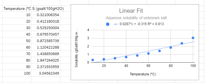
There are several things to note from the graph. First, from a visual perspective the linear function not only does not fit the data, but there is a trend where it is above the line at low and high temperature and below the line in the middle.  The R² value is not near one and most importantly, it predicts a negative solubility as the temperature approaches zero, which is nonsense.  

Power Function: 

\[Y=aX^m\]

Example:  S =aT^m, which can be converted to an equation of the form of a straight line (Y=mX+b) by converting to logs.

\[\begin{align} logS & =log(aT^m) && \text{power function}  \nonumber \\ & =loga + logT^m \nonumber \\ & =loga + mlogT \nonumber \\ logS &= mlogT + loga && \text{linear function} \nonumber \\ y' &= mx' +b' && \text{where y'=logy,  x'=logx  and  b'=logb} \end{align}\]

In the following figure we used Google Sheets to convert the data to log data, and then made two plots, one using a power function fit to the raw data (S,T) and the second using a linear fit with the logS vs. log T data.  These two graphs are different ways of representing the same information.  The slope of the second graph (m=0.983) is the m of S=AT^m of the first graph and the y-intercept (-1.63)= lna from the second equation, so a=10^-1.63=0.023. 

Figure \(\PageIndex{2}\): Power fit on top and the Correlated logS/logT plot on bottom. (CC-BY 4.0; Robert Belford via LibreTexts)

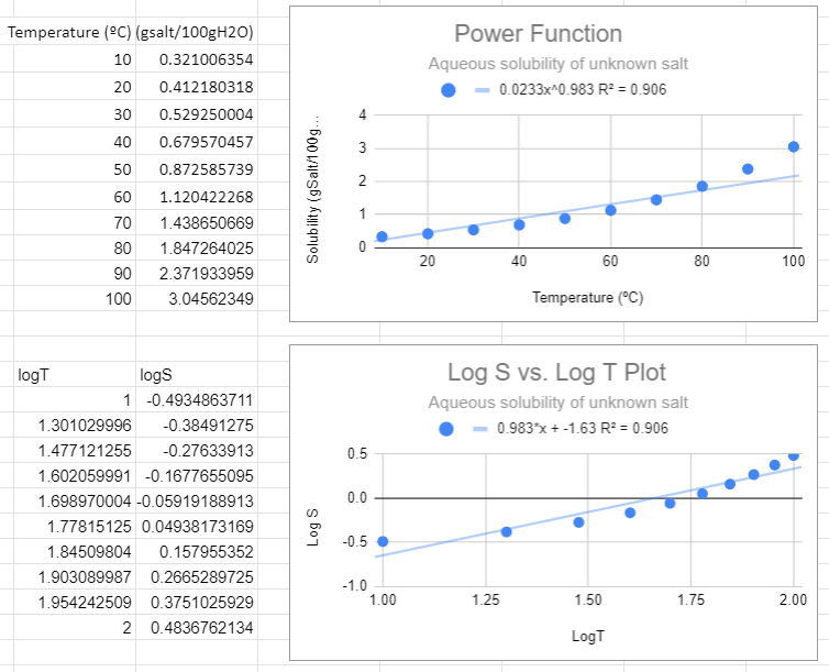
There are several things to notice in the above graphs.  First, from the top graph the  solubility is forced to zero as T goes to zero and this is nonsense, as that would occur no matter what scale you use.  Now students might think a negative logS is an issue, but it is not, that just means the concentration is less than one molar. The R² value is also not close to one, and a student may notice that this power function looks like a linear line, and that is because the value of m is approaching 1 (when m=1 the power function is linear , S=aT +0)

There is one slight of hand going on here that the astute student might catch and that is that we removed the units from the log plots.  Logs can not have units, they are in effect saying how many times you multiplied (or divided) the base by itself to get the number (log₁₀100=2 means 10 times itself 2 times equals 100). When we get to real systems we will need to transform values in exponents (or logs) to dimensionless entities.  This could have been done here by dividing all solubilities by a standard solution with a numeric value of 1 and we will ignore this issue now, but logs do not have units.

 

Exercise \(\PageIndex{1}\)

Transform the power function \(y=5.0x^{3.6}\) to a linear function.

Answer

\(y=5.0x^{3.6}\) is in the power function form \(y=ax^m\)

The linear function form is y=mx+b

b=log(a)

b=log(5.0)=0.70

m=m (The slope does not change)

The linear function is y=3.6x+0.70

Now try practicing converting the linear function to a power function!

Exponential Function: 

\[Y=ae^{mX} \]   

Example  S = ae^mT, which can be converted to a linear function of lnS  to T (not lnT)

\[\begin{align} S & = ae^{mT} && \text{exponential function}\\ lnS & =ln(ae^{mT})  \nonumber \\ & =lna + ln(e^{mT}) \nonumber \\ & =lna + mT\cancel{ln(e)} \nonumber \\ lnS &= mT + lna \\ y'' &= mx +b'' && \text{where y'=logy,  x=x  and  b''=lna} \end{align}\]

An exponential fit of the solubility to temperature gives the same information as a linear fit of the natural log of solubility to temperature, and so the slope of the bottom graph (m=0.025) is the value of m in the exponential function, and the y intercept of the bottom graph gives the pre-expontial, b=-1.39=lna, so a = e^-1.39.=0.249=0.25.

Figure \(\PageIndex{3}\): Exponential plot of solubility as function of temperature.  Note that unlike a power function, this plot does not have to go through the origin. (CC-BY 4.0; Robert Belford via LibreTexts)

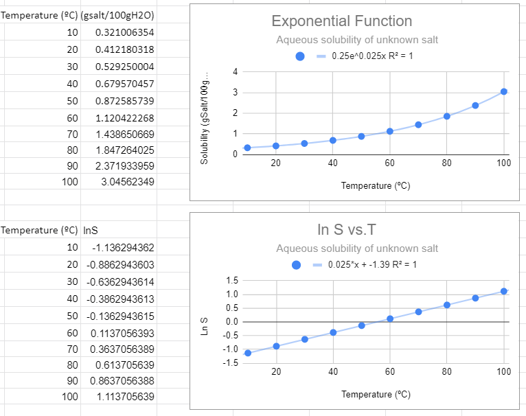
This looks like the best fit. The value of R²=1 and this function makes the most sense in explaining the data.  Also note that when the independent variable (T) equals zero you have e⁰=1, and so the pre-exponential is the value of the solubility at T=0.

Exercise \(\PageIndex{2}\)

Transform the exponential function \(y=5.6e^{7.9x} \) to a linear function.

Answer

\(y=5.6e^{7.9x} \) is in the power function form \(y=ae^{mx} \)

The linear function form is y=mx+b

b=ln(a)

b=ln(5.6)

b=1.7

m=7.9 (The slope does not change)

The linear function is y=7.9x+1.7

Now try practicing converting the linear function to an exponential function!

Graphing Tutorials and Videos

If you are unsure how to do something in this lab, try the resources in Google Workspace

• Sheets Basics
  • Google Workbook
  • Navigating a Google Sheet
  • Making a Google Sheet
  • Copy a Google Sheet
• Google Sheets: Tabs  
  • Make new Tab (Sheet) in Spreadsheet
  • Duplicate a Tab
  • Organizing Tabs
• Format
  • Numbers
  • Decimal Places

• Formulas
  • Basics
  • Simple Mathematical Functions
  • Logarithms

• Charts
  • Charts Basics
  • Insert a Chart
  • Edit a Chart
  • Trendline and Equations
  • Multiple Series