
1.3: Procedures
- Page ID
- 379572
\( \newcommand{\vecs}[1]{\overset { \scriptstyle \rightharpoonup} {\mathbf{#1}} } \)
\( \newcommand{\vecd}[1]{\overset{-\!-\!\rightharpoonup}{\vphantom{a}\smash {#1}}} \)
\( \newcommand{\id}{\mathrm{id}}\) \( \newcommand{\Span}{\mathrm{span}}\)
( \newcommand{\kernel}{\mathrm{null}\,}\) \( \newcommand{\range}{\mathrm{range}\,}\)
\( \newcommand{\RealPart}{\mathrm{Re}}\) \( \newcommand{\ImaginaryPart}{\mathrm{Im}}\)
\( \newcommand{\Argument}{\mathrm{Arg}}\) \( \newcommand{\norm}[1]{\| #1 \|}\)
\( \newcommand{\inner}[2]{\langle #1, #2 \rangle}\)
\( \newcommand{\Span}{\mathrm{span}}\)
\( \newcommand{\id}{\mathrm{id}}\)
\( \newcommand{\Span}{\mathrm{span}}\)
\( \newcommand{\kernel}{\mathrm{null}\,}\)
\( \newcommand{\range}{\mathrm{range}\,}\)
\( \newcommand{\RealPart}{\mathrm{Re}}\)
\( \newcommand{\ImaginaryPart}{\mathrm{Im}}\)
\( \newcommand{\Argument}{\mathrm{Arg}}\)
\( \newcommand{\norm}[1]{\| #1 \|}\)
\( \newcommand{\inner}[2]{\langle #1, #2 \rangle}\)
\( \newcommand{\Span}{\mathrm{span}}\) \( \newcommand{\AA}{\unicode[.8,0]{x212B}}\)
\( \newcommand{\vectorA}[1]{\vec{#1}} % arrow\)
\( \newcommand{\vectorAt}[1]{\vec{\text{#1}}} % arrow\)
\( \newcommand{\vectorB}[1]{\overset { \scriptstyle \rightharpoonup} {\mathbf{#1}} } \)
\( \newcommand{\vectorC}[1]{\textbf{#1}} \)
\( \newcommand{\vectorD}[1]{\overrightarrow{#1}} \)
\( \newcommand{\vectorDt}[1]{\overrightarrow{\text{#1}}} \)
\( \newcommand{\vectE}[1]{\overset{-\!-\!\rightharpoonup}{\vphantom{a}\smash{\mathbf {#1}}}} \)
\( \newcommand{\vecs}[1]{\overset { \scriptstyle \rightharpoonup} {\mathbf{#1}} } \)
\( \newcommand{\vecd}[1]{\overset{-\!-\!\rightharpoonup}{\vphantom{a}\smash {#1}}} \)
\(\newcommand{\avec}{\mathbf a}\) \(\newcommand{\bvec}{\mathbf b}\) \(\newcommand{\cvec}{\mathbf c}\) \(\newcommand{\dvec}{\mathbf d}\) \(\newcommand{\dtil}{\widetilde{\mathbf d}}\) \(\newcommand{\evec}{\mathbf e}\) \(\newcommand{\fvec}{\mathbf f}\) \(\newcommand{\nvec}{\mathbf n}\) \(\newcommand{\pvec}{\mathbf p}\) \(\newcommand{\qvec}{\mathbf q}\) \(\newcommand{\svec}{\mathbf s}\) \(\newcommand{\tvec}{\mathbf t}\) \(\newcommand{\uvec}{\mathbf u}\) \(\newcommand{\vvec}{\mathbf v}\) \(\newcommand{\wvec}{\mathbf w}\) \(\newcommand{\xvec}{\mathbf x}\) \(\newcommand{\yvec}{\mathbf y}\) \(\newcommand{\zvec}{\mathbf z}\) \(\newcommand{\rvec}{\mathbf r}\) \(\newcommand{\mvec}{\mathbf m}\) \(\newcommand{\zerovec}{\mathbf 0}\) \(\newcommand{\onevec}{\mathbf 1}\) \(\newcommand{\real}{\mathbb R}\) \(\newcommand{\twovec}[2]{\left[\begin{array}{r}#1 \\ #2 \end{array}\right]}\) \(\newcommand{\ctwovec}[2]{\left[\begin{array}{c}#1 \\ #2 \end{array}\right]}\) \(\newcommand{\threevec}[3]{\left[\begin{array}{r}#1 \\ #2 \\ #3 \end{array}\right]}\) \(\newcommand{\cthreevec}[3]{\left[\begin{array}{c}#1 \\ #2 \\ #3 \end{array}\right]}\) \(\newcommand{\fourvec}[4]{\left[\begin{array}{r}#1 \\ #2 \\ #3 \\ #4 \end{array}\right]}\) \(\newcommand{\cfourvec}[4]{\left[\begin{array}{c}#1 \\ #2 \\ #3 \\ #4 \end{array}\right]}\) \(\newcommand{\fivevec}[5]{\left[\begin{array}{r}#1 \\ #2 \\ #3 \\ #4 \\ #5 \\ \end{array}\right]}\) \(\newcommand{\cfivevec}[5]{\left[\begin{array}{c}#1 \\ #2 \\ #3 \\ #4 \\ #5 \\ \end{array}\right]}\) \(\newcommand{\mattwo}[4]{\left[\begin{array}{rr}#1 \amp #2 \\ #3 \amp #4 \\ \end{array}\right]}\) \(\newcommand{\laspan}[1]{\text{Span}\{#1\}}\) \(\newcommand{\bcal}{\cal B}\) \(\newcommand{\ccal}{\cal C}\) \(\newcommand{\scal}{\cal S}\) \(\newcommand{\wcal}{\cal W}\) \(\newcommand{\ecal}{\cal E}\) \(\newcommand{\coords}[2]{\left\{#1\right\}_{#2}}\) \(\newcommand{\gray}[1]{\color{gray}{#1}}\) \(\newcommand{\lgray}[1]{\color{lightgray}{#1}}\) \(\newcommand{\rank}{\operatorname{rank}}\) \(\newcommand{\row}{\text{Row}}\) \(\newcommand{\col}{\text{Col}}\) \(\renewcommand{\row}{\text{Row}}\) \(\newcommand{\nul}{\text{Nul}}\) \(\newcommand{\var}{\text{Var}}\) \(\newcommand{\corr}{\text{corr}}\) \(\newcommand{\len}[1]{\left|#1\right|}\) \(\newcommand{\bbar}{\overline{\bvec}}\) \(\newcommand{\bhat}{\widehat{\bvec}}\) \(\newcommand{\bperp}{\bvec^\perp}\) \(\newcommand{\xhat}{\widehat{\xvec}}\) \(\newcommand{\vhat}{\widehat{\vvec}}\) \(\newcommand{\uhat}{\widehat{\uvec}}\) \(\newcommand{\what}{\widehat{\wvec}}\) \(\newcommand{\Sighat}{\widehat{\Sigma}}\) \(\newcommand{\lt}{<}\) \(\newcommand{\gt}{>}\) \(\newcommand{\amp}{&}\) \(\definecolor{fillinmathshade}{gray}{0.9}\)Getting started
Downloads and Forms
Google Sheet Template - this link makes a copy of the lab template that you use to develop your Google Lab Workbook
Google Form - Use the form associated with your lab to submit the URL of your Google Lab Workbook to your instructor through this form
Share Spreadsheet
Sheet Skills
How to turn on link sharing to give Instructor Access and Submit Spreadsheet
- Instructions
-
To turn in your spreadsheet we need to enable link sharing. Your sheet may look slightly different depending on your university but the steps will still be the same.
Open the form your instructor sent you and your copy of the spreadsheet.
- On your Spreadsheet Click Share in the top Right Corner (Figure 1)
- Go down to Get Link and click Change link (Figure 1)
- Change permissions to Editor (Figure 2)
- Press Copy Link (Figure 2)
- Go to the form and fill out your email and Name
- When it asks for your Link to Spreadsheet paste the link we copied in step 4.
- Submit your form
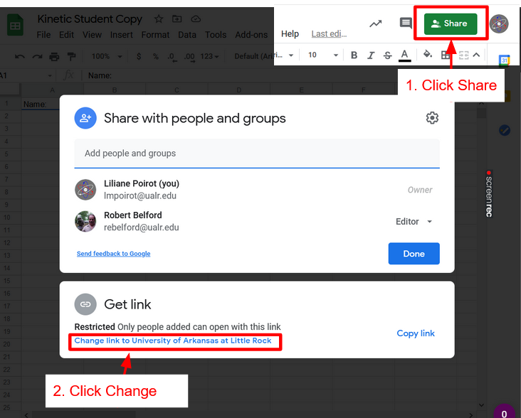
Figure \(\PageIndex{1}\): Click Share at the top Right of your spreadsheet. Then click change link. (CC-BY 4.0; Poirot via LibreTexts) 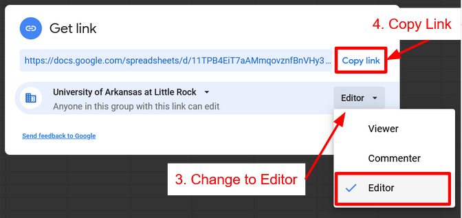
Figure \(\PageIndex{2}\): Change permissions to Editor then Copy Link. (CC-BY 4.0; Poirot via LibreTexts)
Graphing Exercise Procedures
Click Spreadsheet above to get a copy of the spreadsheet. Once that is done click Share Spreadsheet with Instructor, click the link to the Form for your lab and lab section.
Instructions
- Use the solubility data in Table 1.1 to construct seven graphs with Google Sheets
- Follow the formatting suggested in the above videos and tutorials
- axis correctly labeled
- major and minor grid lines are shown
- trendline and the equation for the line of best fit is shown clearly
- Make sure your data and graph are shown side by side on the tab, and the graph is copied to the coverpage
- Submit your Workbook to Adapt by your sections' due date
| Temperature (oC) | Solubility Unknown A (g / 100g H2O) | Solubility Unknown B (g / 100g H2O) |
|---|---|---|
| 30 | 50.8 | 179 |
| 45 | 72.7 | 205 |
| 60 | 104.0 | 230 |
| 75 | 148.9 | 255 |
| 90 | 213.1 | No data available |
Tab 1: Cover Page
- The cover page summarizes all your results and data.
- Fill out your personal information before proceeding to the rest of the lab
- When you are done with each tab you will copy and paste the graphs and resize them to fit in the appropriate box.
- Make sure any orange highlighted cells are filled out before submitting work. These will be graded.
Tab 2: Linear Graph Salt A
From the data in Table 1, create the following graph:
Graph 1: Linear Fit of Temperature vs. solubility for Salt A
Things to keep in mind when making these graphs:
- Label each graph with a title describing the graph and label all axes (don't just accept the automatic label)
- Select the linear regression trend line (y=mx+b) and make sure that you select to show the equation for the line. Move the equation and adjust size so it is clearly visible
Hint! If you set your data range as the entire column (for example A:B instead of A1:B6) your graph will automatically include any new data
Tab 3: Linear Graph Salt B
Duplicate Tab 2 and replace with data from Salt B to make Graph 2: Linear Fit of Temperature vs. solubility for Salt B
Things to keep in mind when making these graphs:
- Check that the labels for your data and on the graph are correct, google doesn't always automatically update them
- Pay attention to the range on your axes, does it fit your data?
Tab 4: Comparison Linear Graph Salt A&B
Create a Chart to compare the two sets of data by creating a multiple series chart.
Tutorial for this multiple series chart
Design Requirements
- Smoothline chart with dashed lines and data points
- Linear regression trendlines for both series with equation and R
Note: a linear fit will only be a good fit (R2 value close to 1) for one of these salts. Once you identify which one is a good fit, you have now created an equation that will allow you to predict the solubility of that salt at another temperature!
Copy and Paste this chart to the Coverpage and size it to fit the correct box. Identify which one is a good fit
Tab 5: Power Functions
For the salt that does not have a linear relationship between temperature and solubility, you will now make graph 4 & 5.
Duplicate the tab of the data you need so you can make your next graphs.
Graph 4: Power function trend line (y=axb) for the nonlinear graph
(You will now need to create a new column in the graph that calculates the log of the values.)
Graph 5: Find then make a plot of log S vs. log T plot (eq. 1.3 or 1.4) and run a linear fit on this graph. Be sure you can relate graph 5 to graph 4 as described in section 1.2 (figures 1.2 & 1.3).
- Show that the slope of a straight line in this graph is equal to the power (m) in graph 4.
- Mathematically show how the y intercept of this graph can be used to determine the pre-exponential term (A) in graph 4
Tab 6: Exponential Functions
For graphs 6 & 7 make another copy of the data you used for graph 4. You will now need to create a new column in the graph that calculates the ln of the values.
Graph 6: Exponential trend line (y=aemx) fit for the nonlinear graph.
- Write the appropriate equation on all graphs.
- Determine which fit is best.
Graph 7: Make a plot of ln S vs. T and run a linear fit on this graph. Be sure you can relate graph 7 to graph 6 as described in section 1.3 (figures 1.4 & 1.5)
- Show that the slope of a straight line in this graph is equal to the power (m) in graph 6.
- Mathematically show how the y intercept of this graph can be used to determine the pre-exponential term (A) in graph 5
TIPs:
- Use these as templates for future graphs by simply copying the graph, then changing the source data and labeling.
- Hence, you'll want to remember where you saved this file so for future labs you can come back and use the template you already created (saving you time)!
Assessment (self-check):
- Do you know the difference between a dependent and independent variable?
- Do you know where to place the dependent variable on graph? Independent variable?
- Can you title a graph properly?
- Can you label all graph components properly?
- Can you use Google sheets to convert data values to logarithm form?
- Do you know when to and when not to include units?
- Do you know how to add and evaluate a trend line (line of best fit) and correlation magnitude (R2)?
- Can you determine the constants of a power function from a linear plot of the appropriate log data values?
- Can you determine the constants of an exponential function from a linear plot of the appropriate data and ln data values?