8.2: Background

Background

In this lab we are going to run a Jobs plot to determine the formation constant for the formation of a coordination complex of iron(II) and 1,10 phenanthroline.  A Jobs plot is similiar to a titration. In acid/base titrations the pH is measured as a function of the amount of titrant (strong acid or base) that is added to the analyte (base or acid). The titration starts with pure analyte, then a buffer is formed while the analyte is the excess reagent and only part of it has been converted to its salt.  At the equivalence point the two reagents are in stoichiometric proportions and upon further addition of titrant the analyte becomes the limiting reagent and the pH is dictated by the excess titrant.

In a pH titration the pH is changing for two reasons.

1. neutralization
2. dilution.

In a Jobs plot the total volume is kept constant and so the reactant and product concentrations are not influenced by dilution. Unlike a titration where you continually add one reactant to another and measure the effect, in a Job's plot each measurement is a unique solution where the mole fraction of reactants are varied.  If a Job's plot had 20 measurements you would need to make 20 different solutions, where each solution represented different mole fraction ratios. Another name for the Job's Plot is the method of continuous variations and in this lab the Job's plot technique will be be applied to the formation of a coordination complex ion. 

Coordination Complexes

Many metal ions have vacant d orbitals that allow them to function as Lewis Acids (electron acceptors) that can react with molecules (or ions) containing lone pairs of electrons, the Lewis bases (electron donors). These reactions can result in the formation of a coordination complex (sections 16.7: & 17.6), which are often highly colored. In this type of reaction the Lewis base is called the Ligand (L) and may be neutral (NH₃, H₂O,...) or charged (Cl^-, NO₂^-, ...).  The sum of the charges of the metal cation and all the ligands bonded to it gives the charge of the coordination complex, which may result in a neutral, cationic (positive) or anionic (negative) complex.  Charged coordination complexes are known as complex ions and are often soluble and highly colored. A complex ion consists of a central metal atom and a specific number of ligands covalently bonded to it, which determines its chemical formula. Water is a typical Lewis base and common aqueous metal ions like Fe⁺²,  Fe⁺³,  Cu⁺² and Al⁺³ ​form complex ions with water, that is, they form covalent bonds with the water, where both electrons come from the water. 

Coordination complexes will be studied in more detail when we get to chapter 20 and for this lab it suffices to know that a complex ion can form from the Lewis Acid-Base reaction between a metal cation and a ligand (sections 16.7: & 17.6). 

Figure \(\PageIndex{1}\): Ball and stick and "pseudo" Lewis dot structure of the hexaaqua iron (III) cation . Nomenclature of these will be covered in section 20.3 and what needs to be noted here is that the water is functioning as a ligand, and forms dative coordinate covalent bonds to the metal ion.  In the Lewis dot structure the two electrons of the lone pair from the water are shown in red and the arrow indicates that both electrons of the covalent bond come from the water, (which is acting as a Lewis base, an electron donor).

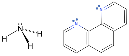
A ligand may be monatomic (Cl^-) or polyatomic (NH₃). For polyatomic ligands the donor atom of the ligand is the atom that has the lone pair of electrons that form the coordinate covalent bond with the metal ion (oxygen is the donor atom of water in figure \(\PageIndex{1}\)). A polyatomic ligand may have more than one donor atom and thus form more than one coordinate covalent bond.  In figure \(\PageIndex{2}\) there are two ligands where nitrogen functions as the donor atoms.  A ligand with one donor atom is classified as a monodentate ligand, a ligand with two donor atoms is a bidentate ligand, and there are polydentate ligands with up to 6 donor atoms. 

Figure \(\PageIndex{2}\): Two Ligands, ammonia (monodentate) and phenanthroline (bidentate)

The resulting coordination complex has a specific number of coordinate covalent bonds, which is the coordination number of the complex.  Figure \(\PageIndex{3}\) shows generic coordination complexes with various numbers of monodentate ligands and one bidentate ligand. The coordination number is only equal to the number of ligands if the ligands are monodentate, and in the case of the bidentate ligand with a formula ML₃ the coordination number (CN) is 6. Typical coordination numbers vary from 2 to 6 and the complexes have geometries similar to the VSEPR geometries we learned about in the first semester of the class.

Figure \(\PageIndex{3}\): Formula and coordination number for different coordination complexes. Note the complex ion on the right involves a bidentate ligand where oxygen is the donor atom and the formula ML₃ results in a coordination number of 6.

In this experiment we will be creating a highly colored complex ion between ferrous iron (Fe⁺²) and a neutral bidentate ligand (figure \(\PageIndex{2}\)).  We will then determine the formula for the complex ion and its formation constant. The generic equation for the formation of a complex with "b" ligands is:

\[M + bL \rightleftharpoons ML_b \]

The above equation results in the following generic formation constant:

\[K_f=\frac{[ML_b]}{[M][L]^b} \]

We will use absorbance spectroscopy and make measurements at a wavelength where the metal and the ligand are both colorless, but the complex ML_b is highly colored, and thus monitor the formation of the complex by the intensity of its color. The technique we will used is called the Job's Plot, or the method of continuous variations.

Job's Plot

A Job's plot is also know as the method of continous variations, where you measure the concentration of the product after varying the mole fractions of the reactants, and then plot the concentration of product as the dependent variable, with the mole fractions as the independent variable.  Since there are only two species there are two scales on the x axis, one for the mole fraction ligand and the other for the mole fraction of the metal, and they are related by the equation  X_M + X_L = 1.  

 

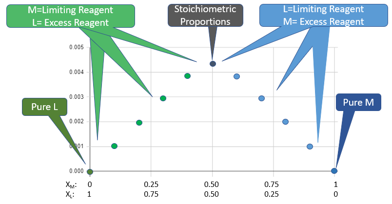Figure \(\PageIndex{4}\): Regions of Job Plot. Note, the scale on the X-axis shows the mole fractions of metal (X_M) and Ligand (X_L), with the fraction varying from pure ligand (left) to pure metal (right).  The peak represents when they are mixed in stoichiometric proportions.  (Belford)

The peak of jobs plot identifies the ratio of ligand to metal at stoichiometric proportions and thus allows one to determine the formula of the coordination complex. One can also look at the ratios of the slopes in regions where the limiting reagent is completely consume and use that to determine the proportions at which they react, and thus the formula of the product.  When doing so it is important to realize that you are not measuring the reactant concentrations but the product concentration, which is plotted as a function of the reactant mole fraction.

Comparing Job's Plot to a Titration

Both titrations and Job's plots start with a pure reactant and then measure some effect from adding a second substance that reacts with the first. In an acid base reaction this is the hydronioum ion concentration (pH).  It should be emphasized that acid-base titrations are only one type of titration, and other types of titrations like redox titrations are common.  In a titration there is only one solution and you make measurements as you successively add the titrant. In the Job's plot each measurement is a different solution. In the titration the concentration of the initial reactant (analyte) is being reduced by two processes, reaction with the titrant and dilution, as the total volume of the solution increases as you add titrant. In the Job's plot you keep the total volume constant while varying the proportions of the different reagents mixed, so in a Job's plot you do not have an analyte and titrant, but start with a solution that is pure reactant "A" and end with one that is pure reactant "B". In both titrations and Job's plots you need a way to measure the progress of the reaction.  In pH titrations this can be down with an indicator or pH meter. In a Job's plot this is often done with spectroscopy because the complexes are often highly colored, while the metal solutions and ligands are often colorless.

Beer's Law

Coordination complexes can be highly colored and we will use a spectrometer to measure the concentration of the coordination complex. According to Beer's Law the concentration is proportional to the absorbance. \[A=\epsilon bc\] where \(\epsilon\) = extinction coefficient, b=path length and c=concentration (experiment 3.2b).  You need to review the use of spectrometers (section 0.3 of the general information) and realize that for the spectrometer we are using, you can only trust Beer's law over the absorbance range of 0.05 to 1.