4.2: Background

This experiment will introduce you to the use of spectrometers, and techniques for using them.  The goal of this lab is to understand the kinetics for the bleaching of crystal violet by sodium hydroxide.  This is done by measuring how the blue color of the crystal violet solution becomes colorless over time 

IMPORTANT

Before Proceeding Read Section 4.5.1-4 (Resources and Further Information) of this experiment.

1. Absorbance Spectroscopy Overview
2. Spectrometer Design
3. Absorbance
4. Beer's Law

In this lab you are responsible for the material in that section. Your prelab questions, postlab quiz and lab activity require you to be familiar with that material. 

 

There are essentially three components to this lab.

1. Obtain an absorbance spectra.  This is a plot of the absorbance as a function of wavelength, and is sort of a fingerprint of a molecule, which is often used as a qualitative technique to identify if a molecule is present.
2. Obtain a Beer's Law plot.  This allows one to determine the concentration of a chemical species as a function of its absorbance.
3. Obtain a kinetics decay plot.  This is a plot of the absorbance as it changes over time, and can be used to determine the kinetics of a reaction. We are actually running this experiment before we cover this material in lecture and using this lab to introduce the concept of kinetics.

Absorbance Spectra

An absorbance spectra is a plot of the light absorbed as it travels through a sample as a function of its wavelength. Figure \(\PageIndex{2}\) shows the spectral characteristics of the spectra of chlorophyll a and chlorophyll b.

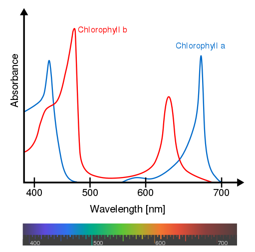figure \(\PageIndex{2}\): Vis spectra of chlorophyll (Wikimedia Commons)

When visible light interacts with a molecule's electrons they absorb the energy of the photons and can be excited from low energy to a higher energy states if the energy gap between the orbitals is equal to the energy of the light absorbed.  In gen chem 1 (section 6.2) we learned that this energy is related to the frequency and wavelength of the light by Planks constant \(E= (h\nu =h\frac{c}{\lambda}\)) and that the intensity (I) of light at a specific frequency was nh\(\nu\).  We studied line spectra of atoms  (section 6.3) where we could identify the atom by its unique absorbance or emission spectrum.  Molecules have more complex orbitals and bonds that are in constant vibrational motion, so their energy gaps are constantly changing and they do not produce a discrete line spectrum like the gaseous atom, but a sort of blurring of the lines as seen in figure \(\PageIndex{2}\)), where each peak is associated with an electronic transition.  In the line spectra we only noted if light was absorbed (or emitted) at a wavelength, but in molecular spectroscopy we are also concerned with the number of photons absorbed by the molecule at that wavelength. So the Y-axis of the spectrum in figure  \(\PageIndex{2a}\) is theaAbsorbance (A), which is logarithmically related to the reduction in intensity of light as it travels through the sample.

\[A=log\frac{I_0}{I_t}\]

where, 

A=Absorbance
I₀= light intensity entering sample
I_t = light intensity leaving (transmitted through) sample

This equation is derived in the Resources and Further Information (section 4.5.4) of this experiment.  It should be noted that what is measured by the spectrometer is the intensity of light, and there is a small range of absorbances where we can trust the value of the data from our spectrometer. The rule of thumb we will use is that we only trust Absorbance values between 0.05 and 1.0.  It is important to realize that any instrument has a range for which it is calibrated, and you need to know the accuracy (and precision) of any instrument you use in the lab.

Beer's Law

Beer's law is followed if a plot of the Absorbance at a specific wavelength vs. the concentration of a molecule that absorbs light at that wavelength is linear. Figre \(\PageIndex{3}\) shows a plot that follows Beer's Law, which is commonly expressed in the form of:
\[A=\epsilon bc\]

where

• \(\epsilon\)= the extinction coefficient 
• b=path length 
• c=concentration

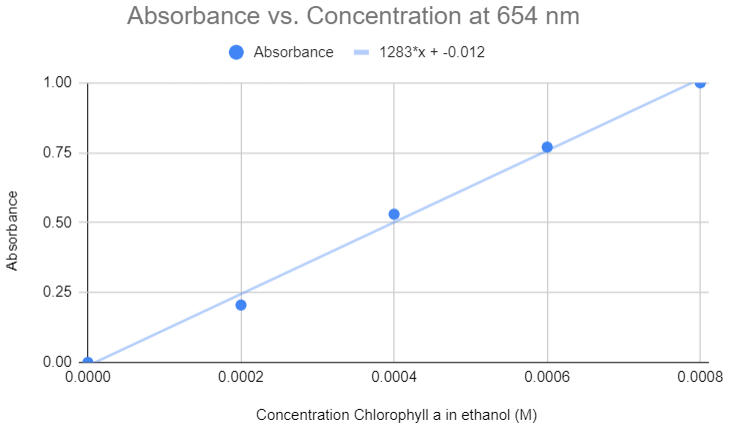Figure \(\PageIndex{3}\): Linear Plot of Absorbance vs Concentration. (Belford)

Beer's Law is derived in section 4.5.4 of this lab. Deeper Dive 4.5.1 shows the calculus and you should not that mathematically this is the same kind of relationship that results in first order reaction equations that we are studying in the lecture.  That is, a logarithmic relationship arises when the rate at what something changes is proportional to the thing itself.  In first order kinetics the rate of change in concentration as a function of time is proportional to the concentration, \(\frac{\Delta [A]}{\Delta t}=-k[A]\) and here it is the change in intensity of light as a travels is proportional to the intensity of light \(\frac{\Delta [I]}{\Delta x}=-k[I]\).  As you advance in your studies you will frequently see these kinds of logarithmic relationships and you need to be comfortable with them (calculus is not a prerequisite for this class, but the equations we use come from the calculus, and you need to know that).

What is very important to realize in the lab that is that your instrument has a range where it can accurately make a measurement, and in this lab we only trust absorbance values between 0.05 and 1.0. 

Exercise \(\PageIndex{1}\)

The extinction coefficient of a sample at 654 nm is 100000 cm^-1M^-1. What is the concentration of an unknown sample if it had an absorbance of 1.00 in a cuvette with a 1.0 cm path length?

Answer

\[A=\epsilon bc\]

\(\epsilon\)= 100000 cm^-1M^-1

b=1 cm

c=?

1.00=(100000 cm^-1M^-1)(1 cm)(c)

c=1.00/((100000 cm^-1M^-1)(1 cm))

c=0.000010 M

Kinetics Decay Plots

In lecture we will first study the differential rate laws and then derive the integrated rate laws from them.  The integrated rate laws are easier to experimentally understand, and so we are going to run the lab on the integrated rate laws before doing the differential rate laws experiment. The rate of reaction describes how fast a product is produced or a reactant is consumed (section 14.1) and the rate law (section 14.3) is a power function.

\[A \rightarrow Products \\ R=k[A]^m \\ \; \\ \text{describing the rate in terms of the reactant concentration} \\ \;\\ \frac{\Delta [A]}{\Delta t}=-k[A]^m\]

As the above equation has a power, we would need to do a log/log plot, where the dependent variable (Y-axis) would be the log of the rate (\(\frac{\Delta [A]}{\Delta t}\)) and the independent variable (X-axis) would be the log of the concentration (log[A]), and we will run those experiments next week. 

The integrated rate laws are covered in section 14.4 and simply describe how the concentration of a reactant changes over time. That is, we solve the following equation for [A] and time

\[\frac{\Delta [A]}{\Delta t}=-k[A]^m\]

This requires calculus and we are only going to look at three solutions, which are for the values of m = 0,1 or 2. Calculus is not a prerequisite for this course, but if you are interested the relevant integrals are in section 4.5.5 . 

Zero Order Reaction

\[Rate=\frac{\Delta[A]}{\Delta{t}}=-k[A]^0=-k\]

When integrated, there is a direct linear relationship between the concentration and time

\[A]_t = -kt + [A]_0\]

 

 

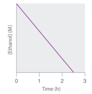Figure \(\PageIndex{1}\): For a Zero Order Reaction a plot of the concentration vs. time is linear.

 

First Order Reaction

\[Rate=\frac{\Delta[A]}{\Delta{t}}=-k[A]^1=-k[A] \]

When integrated this results in a linear relationship for the natural log of the concentration as a function of time

\[ln[A]_t = -kt + ln[A]_0\]

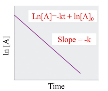Figure \(\PageIndex{1}\): For a Zero Order Reaction a plot of the concentration vs. time is linear.

 

Second Order Reaction

\[Rate=\frac{\Delta [A]}{\Delta{t}}=-k[A]^2\]

When integrated this results in a linear relationship for the reciprocal log of the concentration as a function of time

\[\frac{1}{[A]_t} = kt + \frac{1}{[A]_0}\]

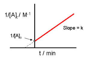Figure \(\PageIndex{1}\): For a Zero Order Reaction a plot of the concentration vs. time is linear.

 

Summary of Rate Laws

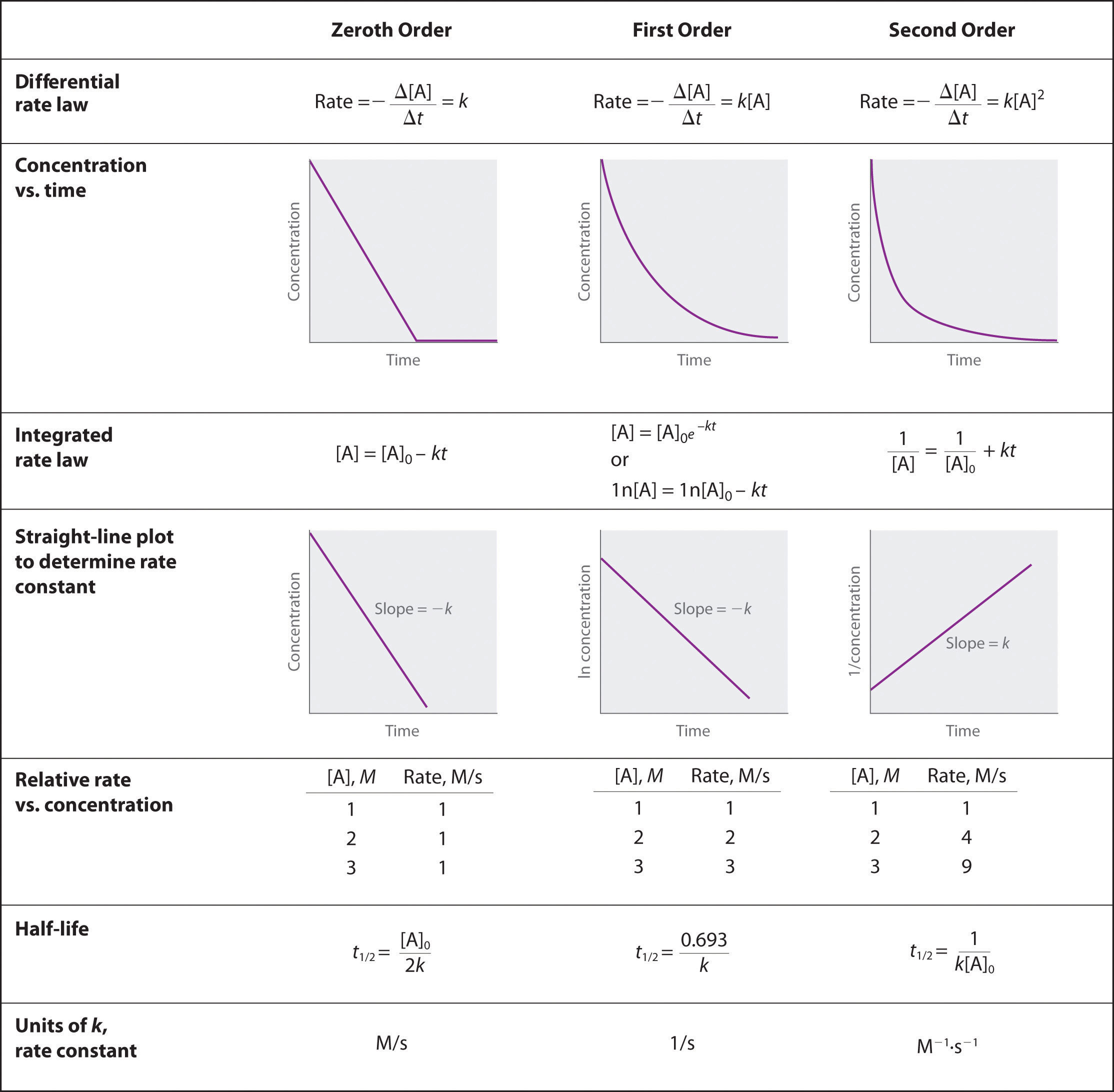
The above table summarizes the material in sections 14.4.3.and 14.4.4

 

The Kinetics Experiment

This lab will involve the bleaching of crystal violet dye by sodium hydroxide

\[\underbrace{CV^+}_{blue} + OH^- \rightarrow \underbrace{CVOH}_{clear}\]

Which has the rate law of

\[R=k[CV^+][OH^-]\]

In this experiment the [CV⁺]= 0.00002M and the [OH^-]=0.10M, which means the [CV⁺] is 5000 times more concentrated than the hydroxide, and so the concentration of the hydroxide stays constant (by being in such excess it is effectively zero order and does not change over the course of the reaction).  So the rate law reduces to

\[R=k[CV^+]\]

In this lab you will mix 10 mL of the CV with mix with 10 mL of the sodium hydroxide and immediately transfer to the spectrometry that is set up to collect data every 5 seconds.  Your goal is to get data for the full range of absorbances from 1.0 to 0.05.  There is no problem if your initial absorbance is greater than 1.0, just do not use that data when you make your graphs.  But there are problems if your initial values are too low, as all plots will start to look linear as you approach 0.05 absorbance.  You will get the clearest results if your data spans the range the instrument is best suited to measure.