11.2B: Separation Theory

 

Raoult's and Dalton's Laws

Distillation of mixtures may or may not produce relatively pure samples. Distillation involves boiling a solution and condensing its vapors followed by collecting the condensation and analyzing the product. The composition of the distillate is identical to the composition of the vapors. Several equations can be used to describe the composition of vapor produced from a solution.

Raoult's law states that a compound's vapor pressure is lessened when it is part of a solution, and is proportional to its molar composition. Raoult's law is shown in Equation \ref{1}. The equation means that a solution containing \(80 \: \text{mol}\%\) compound "A" and \(20 \: \text{mol}\%\) of another miscible component would at equilibrium produce \(80\%\) as many particles of compound A in the gas phase than if compound A were in pure form.

\[ P_A = P_A^o \chi_A \label{1}\]

where \(P_A^o\) is the vapor pressure³ of a sample of pure A, and \(\chi_A\) is the mole fraction of \(A\) in the mixture.

Dalton's law of partial pressures states that the total pressure in a closed system can be found by addition of the partial pressures of each gaseous component. Dalton's law is shown in Equation \ref{2}.

\[P_\text{total} = P_A + P_B \label{2}\]

A combination of Raoult's and Dalton's laws is shown in Equation \ref{3}, which describes the vapor produced by a miscible two-component system (compounds A + B). This combined law shows that the vapors produced by distillation are dependent on each component's vapor pressure and quantity (mole fraction).

\[P_\text{solution} = P_A^o \chi_A + P_B^o \chi_B \label{3}\]

A compound's vapor pressure reflects the temperature of the solution as well as the compound's boiling point. As temperature increases, a greater percentage of molecules have sufficient energy to overcome the intermolecular forces (IMF's) holding them in the liquid phase. Therefore, a compound's vapor pressure always increases with temperature (see Table 5.2), although not in a linear fashion.

Table 5.2: Vapor pressure data for selected compounds.\(^4\)

Compound	Boiling Point (ºC)	Vapor Pressure at 0 ºC	Vapor Pressure at 20 ºC
Diethyl Ether	34.6	183 mmHg	439 mmHg
Methanol	64.7	30 mmHg	94 mmHg
Benzene	80.1	24.5 mmHg	75 mmHg
Toluene	110.6	6.8 mmHg	22 mmHg

When comparing two compounds at the same temperature, the compound with weaker IMF's (the one with the lower boiling point) should more easily enter the gas phase. Therefore, at any certain temperature, a compound with a lower boiling point always has a greater vapor pressure than a compound with a higher boiling point (see Table 5.2). This last concept is the cornerstone of distillation theory.

A compound with a lower boiling point always has a greater vapor pressure than a compound with a higher boiling point

Distilling Temperatures

A pure compound distills at a constant temperature, its boiling point. When distilling mixtures, however, the temperature does not often remain steady. This section describes why mixtures distill over a range of temperatures, and the approximate temperatures at which solutions can be expected to boil. These concepts can be understood by examination of the equation that describes a solution's vapor pressure (Equation (6)) and distillation curves.

\[P_\text{solution} = P_A + P_B = P^o_A \chi_A + P^o_B \chi_B \label{6}\]

Imagine an ideal solution that has equimolar quantities of compound "A" (b.p. = \(50^\text{o} \text{C}\)) and compound "B" (b.p. = \(100^\text{o} \text{C}\)). A common misconception is that this solution will boil at \(50^\text{o} \text{C}\),at the boiling point of the lower-boiling compound. The solution does not boil at A's boiling point because A has a reduced partial pressure when part of a solution. In fact, the partial pressure of A at \(50^\text{o} \text{C}\) would be half its normal boiling pressure, as shown in Equation \ref{7}:

\[\text{At } 50^\text{o} \text{C}: \: \: \: \: \: P_A = \left( 760 \: \text{torr} \right) \left( 0.50 \right) = 380 \: \text{torr} \label{7}\]

Since the partial pressures of A and B are additive, the vapor contribution of B at \(50^\text{o} \text{C}\) is also important. The partial pressure of B at \(50^\text{o} \text{C}\) would equal its vapor pressure at this temperature multiplied by its mole fraction (0.50). Since B is below its boiling point \(\left( 100^\text{o} \text{C} \right)\), its vapor pressure would be smaller than \(760 \: \text{torr}\), and the exact value would need to be looked up in a reference book. Let's say that the vapor pressure of B at \(50^\text{o} \text{C}\) is 160 torr.

At 50ºC:

\[ P_B = \left( 160 \: \text{torr} \right) \left( 0.50 \right) = 80 \: \text{torr} \label{8}\]

The solution boils when the combined pressure of the components equals the atmospheric pressure (let's assume \(760 \: \text{torr}\) for this calculation). This equimolar solution would therefore not boil at \(50^\text{o} \text{C}\), as its combined pressure is less than the external pressure of \(760 \: \text{torr}\) (Equation \ref{9}).

At 50 ºC:

\[\begin{align} P_\text{solution} &= P_A + P_B \\[4pt] &= \left( 380 \: \text{torr} \right) + \left( 80 \: \text{torr} \right) \\[4pt] &= 460 \: \text{torr} \label{9} \end{align}\]

The initial boiling point of this solution is \(66^\text{o} \text{C}\), which is the temperature where the combined pressure matches the atmospheric pressure (Equation \ref{10}, note: all vapor pressures would have to be found in a reference book).

At 66 ºC:

\[\begin{align} P_\text{solution} &= P^o_A \chi_A + P^o_B \chi_B \\[4pt] &= \left( 1238 \: \text{torr} \right) \left( 0.5 \right) + \left( 282 \: \text{torr} \right) \left( 0.5 \right) \\[4pt] &= \left( 619 \: \text{torr} \right) + \left( 141 \: \text{torr} \right) = 760 \: \text{torr} \label{10} \end{align}\]

These calculations demonstrate that a solution's boiling point occurs at a temperature between the component's boiling points.\(^5\).

This can also be seen by examination of the distillation curve for this system, where the solution boils when the temperature reaches position a in Figure 5.15a, a temperature between the boiling point of the components.

It is important to realize that mixtures of organic compounds containing similar boiling points (\(\Delta\) b.p. \(< 100^\text{o} \text{C}\)) boil together. They do not act as separate entities (not "A boils at \(50^\text{o} \text{C}\), then B boils at \(100^\text{o} \text{C}\)").

Figure 5.15: a) Distillation curve for a two-component mixture of A (b.p. \(50^\text{o} \text{C}\)) and B (b.p. \(100^\text{o} \text{C}\)), b) Additional markings.

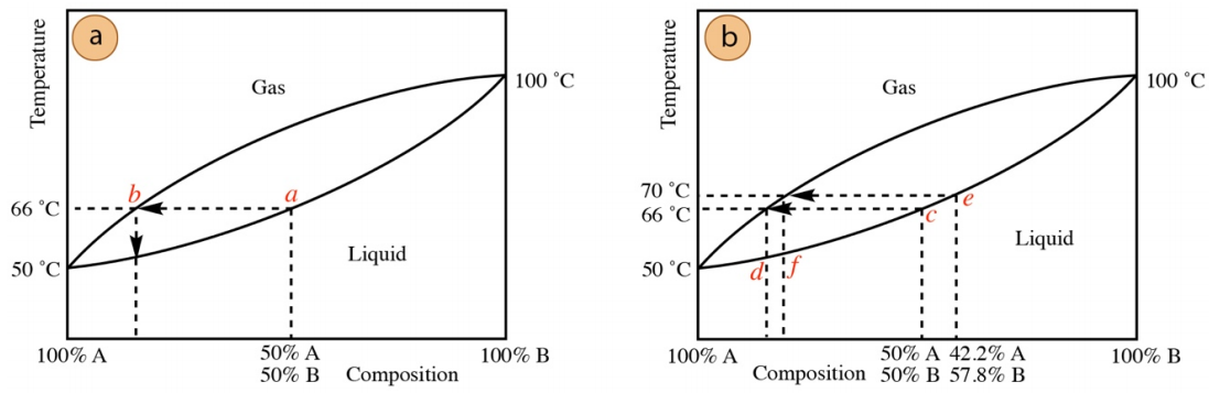
The mixture in this example begins boiling at \(66^\text{o} \text{C}\), but after a period of time boiling would cease if maintained at this temperature. This happens because the composition of the distilling pot changes over time. Since distillation removes more of the lower boiling A, the higher boiling B will increase percentagewise in the distilling pot. Imagine that after some material has distilled, the distilling pot is now \(42.2\%\) A and \(57.8\%\) B. This solution no longer boils at \(66^\text{o} \text{C}\), as shown in Equation \ref{11}.

At 66 ºC:

\[\begin{align} P_\text{solution} &= P^o_A \chi_A + P^o_B \chi_B \\[4pt] &= \left( 1238 \: \text{torr} \right) \left( 0.422 \right) + \left( 282 \: \text{torr} \right) \left( 0.578 \right) \\[4pt] &= \left( 522 \: \text{torr} \right) + \left( 163 \: \text{torr} \right) \\[4pt] &= 685 \: \text{torr} \label{11} \end{align}\]

At the new composition in this example, the temperature must be raised to 70 ºC to maintain boiling, as shown in Equation \ref{12}. This can also be shown by examination of the distillation curve in Figure 5.15b, where boiling commences at temperature c, but must be raised to temperature e as the distilling pot becomes more enriched in the higher boiling component (shifts to the right on the curve).

At 70 ºC:

\[\begin{align} P_\text{solution} &= P^o_A \chi_A + P^o_B \chi_B \\[4pt] &= \left( 1370 \: \text{torr} \right) \left( 0.422 \right) + \left( 315 \: \text{torr} \right) \left( 0.578 \right) \\[4pt] &= \left( 578 \: \text{torr} \right) + \left( 182 \: \text{torr} \right) \\[4pt] &= 760 \: \text{torr} \label{12} \end{align} \]

These calculations and analysis of distillation curves demonstrate why a mixture distills over a range of temperatures:\(^6\) as the composition in the distilling pot changes with time (which affects the mole fraction or the x-axis on the distillation curve), the temperature must be adjusted to compensate. These calculations also imply why a pure compound distills at a constant temperature: the mole fraction is one for a pure liquid, and the distilling pot composition remains unchanged during the distillation.

The calculations and distillation curves in this section enable discussion of another aspect of distillation. The partial pressures of each component at the boiling temperatures can be directly correlated to the composition of the distillate. Therefore, the distillate at \(66^\text{o} \text{C}\) is \(81 \: \text{mol}\%\) A (\(100\% \times 619 \: \text{torr}/760 \: \text{torr}\), see Equation \ref{10}) while the distillate at \(70^\text{o} \text{C}\) is \(76 \: \text{mol}\%\) A (\(100\% \times 578 \: \text{torr}/760 \: \text{torr}\), see Equation \ref{12}). The initial distillate contains the greatest quantity of the lowest boiling component, and the distillate degrades in purity as the distillation progresses. This can also be seen in the distillation curve in Figure 5.15b, where the initial distillate composition corresponds to position d (purer), while the distillate at \(70^\text{o} \text{C}\) corresponds to position f (less pure).

\(^3\)Recall that vapor pressure is the partial pressure of a compound formed by evaporation of a pure liquid into the headspace of a closed container.

\(^4\)Data from Handbook of Chemistry and Physics, 50\(^\text{th}\) ed., CRC Press, Cleveland, 1970, p. 148.

\(^5\)Azeotropic solutions do not follow this same pattern, as they do not obey Raoult's law.

\(^6\)Azeotropic solutions again do not follow this generalization, and instead boil at a constant temperature.

\(^7\)J. A. Dean, Lange's Handbook of Chemistry, 15\(^\text{th}\) ed., McGraw-Hill, 1999, Sect. 5.78 and 5.79.