5: Acid Strength
- Page ID
- 204129
\( \newcommand{\vecs}[1]{\overset { \scriptstyle \rightharpoonup} {\mathbf{#1}} } \)
\( \newcommand{\vecd}[1]{\overset{-\!-\!\rightharpoonup}{\vphantom{a}\smash {#1}}} \)
\( \newcommand{\id}{\mathrm{id}}\) \( \newcommand{\Span}{\mathrm{span}}\)
( \newcommand{\kernel}{\mathrm{null}\,}\) \( \newcommand{\range}{\mathrm{range}\,}\)
\( \newcommand{\RealPart}{\mathrm{Re}}\) \( \newcommand{\ImaginaryPart}{\mathrm{Im}}\)
\( \newcommand{\Argument}{\mathrm{Arg}}\) \( \newcommand{\norm}[1]{\| #1 \|}\)
\( \newcommand{\inner}[2]{\langle #1, #2 \rangle}\)
\( \newcommand{\Span}{\mathrm{span}}\)
\( \newcommand{\id}{\mathrm{id}}\)
\( \newcommand{\Span}{\mathrm{span}}\)
\( \newcommand{\kernel}{\mathrm{null}\,}\)
\( \newcommand{\range}{\mathrm{range}\,}\)
\( \newcommand{\RealPart}{\mathrm{Re}}\)
\( \newcommand{\ImaginaryPart}{\mathrm{Im}}\)
\( \newcommand{\Argument}{\mathrm{Arg}}\)
\( \newcommand{\norm}[1]{\| #1 \|}\)
\( \newcommand{\inner}[2]{\langle #1, #2 \rangle}\)
\( \newcommand{\Span}{\mathrm{span}}\) \( \newcommand{\AA}{\unicode[.8,0]{x212B}}\)
\( \newcommand{\vectorA}[1]{\vec{#1}} % arrow\)
\( \newcommand{\vectorAt}[1]{\vec{\text{#1}}} % arrow\)
\( \newcommand{\vectorB}[1]{\overset { \scriptstyle \rightharpoonup} {\mathbf{#1}} } \)
\( \newcommand{\vectorC}[1]{\textbf{#1}} \)
\( \newcommand{\vectorD}[1]{\overrightarrow{#1}} \)
\( \newcommand{\vectorDt}[1]{\overrightarrow{\text{#1}}} \)
\( \newcommand{\vectE}[1]{\overset{-\!-\!\rightharpoonup}{\vphantom{a}\smash{\mathbf {#1}}}} \)
\( \newcommand{\vecs}[1]{\overset { \scriptstyle \rightharpoonup} {\mathbf{#1}} } \)
\( \newcommand{\vecd}[1]{\overset{-\!-\!\rightharpoonup}{\vphantom{a}\smash {#1}}} \)
\(\newcommand{\avec}{\mathbf a}\) \(\newcommand{\bvec}{\mathbf b}\) \(\newcommand{\cvec}{\mathbf c}\) \(\newcommand{\dvec}{\mathbf d}\) \(\newcommand{\dtil}{\widetilde{\mathbf d}}\) \(\newcommand{\evec}{\mathbf e}\) \(\newcommand{\fvec}{\mathbf f}\) \(\newcommand{\nvec}{\mathbf n}\) \(\newcommand{\pvec}{\mathbf p}\) \(\newcommand{\qvec}{\mathbf q}\) \(\newcommand{\svec}{\mathbf s}\) \(\newcommand{\tvec}{\mathbf t}\) \(\newcommand{\uvec}{\mathbf u}\) \(\newcommand{\vvec}{\mathbf v}\) \(\newcommand{\wvec}{\mathbf w}\) \(\newcommand{\xvec}{\mathbf x}\) \(\newcommand{\yvec}{\mathbf y}\) \(\newcommand{\zvec}{\mathbf z}\) \(\newcommand{\rvec}{\mathbf r}\) \(\newcommand{\mvec}{\mathbf m}\) \(\newcommand{\zerovec}{\mathbf 0}\) \(\newcommand{\onevec}{\mathbf 1}\) \(\newcommand{\real}{\mathbb R}\) \(\newcommand{\twovec}[2]{\left[\begin{array}{r}#1 \\ #2 \end{array}\right]}\) \(\newcommand{\ctwovec}[2]{\left[\begin{array}{c}#1 \\ #2 \end{array}\right]}\) \(\newcommand{\threevec}[3]{\left[\begin{array}{r}#1 \\ #2 \\ #3 \end{array}\right]}\) \(\newcommand{\cthreevec}[3]{\left[\begin{array}{c}#1 \\ #2 \\ #3 \end{array}\right]}\) \(\newcommand{\fourvec}[4]{\left[\begin{array}{r}#1 \\ #2 \\ #3 \\ #4 \end{array}\right]}\) \(\newcommand{\cfourvec}[4]{\left[\begin{array}{c}#1 \\ #2 \\ #3 \\ #4 \end{array}\right]}\) \(\newcommand{\fivevec}[5]{\left[\begin{array}{r}#1 \\ #2 \\ #3 \\ #4 \\ #5 \\ \end{array}\right]}\) \(\newcommand{\cfivevec}[5]{\left[\begin{array}{c}#1 \\ #2 \\ #3 \\ #4 \\ #5 \\ \end{array}\right]}\) \(\newcommand{\mattwo}[4]{\left[\begin{array}{rr}#1 \amp #2 \\ #3 \amp #4 \\ \end{array}\right]}\) \(\newcommand{\laspan}[1]{\text{Span}\{#1\}}\) \(\newcommand{\bcal}{\cal B}\) \(\newcommand{\ccal}{\cal C}\) \(\newcommand{\scal}{\cal S}\) \(\newcommand{\wcal}{\cal W}\) \(\newcommand{\ecal}{\cal E}\) \(\newcommand{\coords}[2]{\left\{#1\right\}_{#2}}\) \(\newcommand{\gray}[1]{\color{gray}{#1}}\) \(\newcommand{\lgray}[1]{\color{lightgray}{#1}}\) \(\newcommand{\rank}{\operatorname{rank}}\) \(\newcommand{\row}{\text{Row}}\) \(\newcommand{\col}{\text{Col}}\) \(\renewcommand{\row}{\text{Row}}\) \(\newcommand{\nul}{\text{Nul}}\) \(\newcommand{\var}{\text{Var}}\) \(\newcommand{\corr}{\text{corr}}\) \(\newcommand{\len}[1]{\left|#1\right|}\) \(\newcommand{\bbar}{\overline{\bvec}}\) \(\newcommand{\bhat}{\widehat{\bvec}}\) \(\newcommand{\bperp}{\bvec^\perp}\) \(\newcommand{\xhat}{\widehat{\xvec}}\) \(\newcommand{\vhat}{\widehat{\vvec}}\) \(\newcommand{\uhat}{\widehat{\uvec}}\) \(\newcommand{\what}{\widehat{\wvec}}\) \(\newcommand{\Sighat}{\widehat{\Sigma}}\) \(\newcommand{\lt}{<}\) \(\newcommand{\gt}{>}\) \(\newcommand{\amp}{&}\) \(\definecolor{fillinmathshade}{gray}{0.9}\)Objectives
- To determine the difference between a strong and a concentrated acid.
- To determine the difference between a weak and a dilute acid.
- To determine the relationship between ionization and pH.
While pure acids are molecular compounds, when they are placed in water the molecules dissociate and form ionic solutions composed of hydronium ions \(\ce{H_{3}O^{+}}\) and the counter anion \(\ce{A^{-}}\).
\[\ce{HA} (aq) + \ce{H_{2}O} (l) \ce{<=>} \ce {H_{3}O^{+}} (aq) + \ce {A^{-}} (aq) \label {1} \]
The presence of the hydronium ion is the basis for determining the pH of the solution.
\[pH=-\log[\ce{H_{3}O^{+}}]\label{2}\]
Using the apparatus with the pH sensor attached will allow you to collect data for the value of the pH in each solution. This will give you information on the concentration of hydronium ions in solution.
Conductivity measures the ability of current to be conducted by a solution. Because it is the ions in the solution that carry current, the more ions there are, the higher the conductivity will be. Thus, conductivity is a measure of the number of ions in a solution.
You will be preparing 0.10 M, 0.010 M, 0.0010 M, and 0.00010 M solutions of hydrochloric acid \(\ce{HCl}\), acetic acid \(\ce{C_{2}H_{4}O_{2}}\), and mandelic acid \(\ce{C_{8}H_{8}O_{3}}\).
Pre Lab Video
Procedure
Safety And Waste Disposal
- The solutions will be sufficiently dilute and as such can be disposed of in the sink.
Part I: Preparing Solutions
Step 1
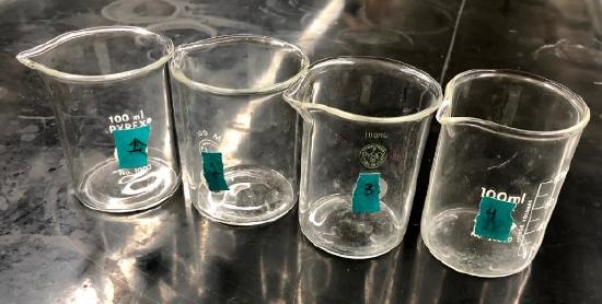 Label 4 small beakers (100 or 150 mL) 0.10 M (Beaker 1), 0.010M (Beaker 2), 0.0010 M (Beaker 3), and 0.00010 M (Beaker 4). Be sure to identify the formula or name of the acid on each label.
Step 2
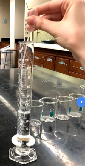 Place 50.0 mL of one of your 0.10 M acid solutions into Beaker 1.
Step 3
 Into each of the three remaining Beakers (2 – 4) add 45 mL of deionized water.
Step 4

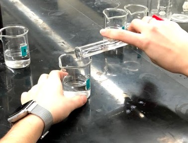 Using a graduated cylinder, add 5.0 mL of the acid in Beaker 1 into Beaker 2 and mix THOROUGHLY.
Step 5
Using a graduated cylinder, add 5.0 mL of the acid in Beaker 2 into Beaker 3 and mix THOROUGHLY.
Step 6
Using a graduated cylinder, add 5.0 mL of the acid in Beaker 3 into Beaker 4 and mix THOROUGHLY.
Part II: Measuring pH
Note
- The pH electrode bulbs are made of glass. They are very fragile. Use extreme care.
- Measure the pH of each of your acids three times rinsing the sensor between readings.
Step 1
Connect the pH Sensor to LabQuest in Channel 1 (CH1).
Step 2
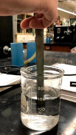 Use about 100 mL of distilled water in a 250 mL beaker to rinse the electrode.
Step 3
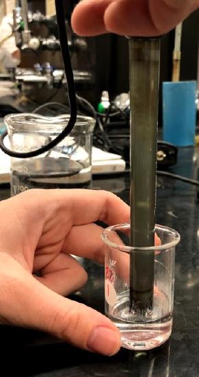 Starting with the 0.00010 M solution, pour about 10 mL of the test solution into a clean 50 mL beaker and use it to thoroughly rinse the electrode.
Step 4
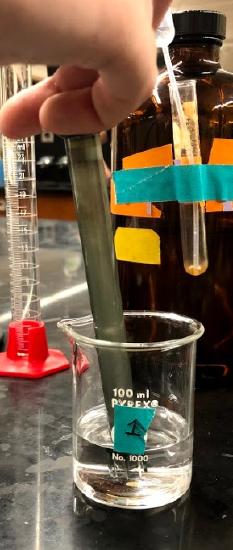 Place the pH electrode in the remaining amount of acid in the beaker. Swirl the solution vigorously. Readings may drift without proper swirling! When the pH reading stabilizes, record the value in your notebook.
Step 5
Repeat with the remaining solutions to determine pH working from the most dilute to the most concentrated beaker.
Step 6
When you are finished, rinse the sensor with distilled water and return it to the sensor soaking solution.
Part III: Measuring Conductivity
Note
You cannot use the conductivity sensor and pH sensor at the same time.
Step 1
Attach the conductivity sensor to the LabQuest in Channel 2 (CH2). Move the range selector switch on the conductivity sensor box to “0-20000 \(\mu\)S/cm” (the largest range).
Step 2
Rinse the sensor with distilled water and pat dry. Do not push the paper towel through the cavity in the probe, but gently tap to remove any droplets of water.
Step 3
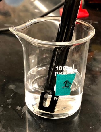 Test only the 0.1 M solutions of each acid. Dip the probe into the solution and swirl the solution. Wait 5 seconds for the conductivity to stabilize. Record the value in your notebook.
Step 4
Rinse and dry the sensor.
Calculations
Step 1
Calculate the average values for the pH of all the acid solutions at each concentration. Record the values on your notebook
Step 2
Open Windows Excel and enter the data on initial concentration and pH for the three acids.
Step 3
Plot pH vs –log (HA)o for each acid (three plots). Use a linear trend line and add the equation along with the \(R^{2}\) value, to the graph. Print these plots.
Step 4
Calculated the experimental \([\ce{H_{3}O^{+}}]\) for all the solutions.
Step 5
Calculate % ionization
\[ \%\: ionization=\frac{[\ce{H_{3}O^{+}}]}{(HA)_{o}}\label{3}\]
Step 6
Calculate, using the appropriate equations, the theoretical \([\ce{H_{3}O^{+}}]\) in each solution. For the weak acids, you will need the values of \(K_{a}\) you found in prelab.
Step 7
Calculate the theoretical pH based on the theoretical \([\ce{H_{3}O^{+}}]\)

