0.1.2: Probability Functions

Saint Mary's College: CHEM 342
Bioinorganic Chemistry
Spring 2020: Dr. Kathryn Haas

Agenda   ●   Readings   ●  Worksheets   ●  Essays  ●  WiSEWIKI

---

A note from Dr. Haas: At this point, I hope you've held on to the idea that the electron's behavior (its location and energy) is described by the Schrödinger equation, a mathematical function. Although a full understanding of the Schrödinger equation is outside the scope of this course, I do want you to have a conceptual understanding of what an orbital is. I hope that you understand the following:

• A three-dimensional plot of the Schrödinger equation (function) is an atomic orbital.
• An atomic orbital is the most probable location of an electron around a nucleus.
• The solution, or plotting of, the Schrödinger equation requires quantum numbers.

So, the shapes of atomic orbitals represent three-dimensional plots of probability. It is sometimes useful to also plot the probability in two dimensions. Two dimensional plots of electron probability are called radial probability functions, where the word "radial" comes from radius (i.e. the function depends on the radius or distance from the nucleus). I have described the Schrödinger equation and radial probability functions in more detail in another course (see further reading below). For now, I want to introduce them to you at a conceptual level because they will become important in this course soon.

---

For now, it's sufficient to think of Radial Probability Functions as plots of orbital density depending on the distance from the nucleus. Study the figure below.

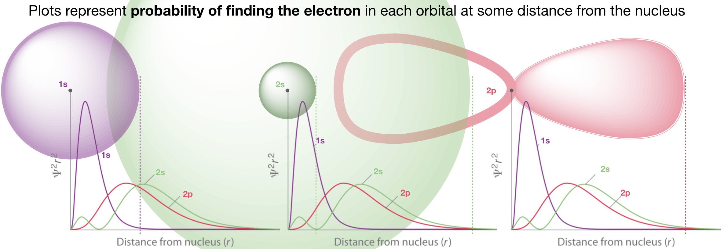
Figure \(\PageIndex{1}\). The radial probability functions are the plots shown. The plots in the left, middle, and right panels are identical and each shows the radial probability of the 1s, 2s, and 2p orbitals. A cartoon of the 1s orbital is overlaid on the left panel, a cartoon of the 2s orbital is shown overlaid on the middle panel, and a cartoon of the 2p orbital is shown overlaid on the right panel. (CC-BY-NC-SA; Kathryn Haas)

Exercises

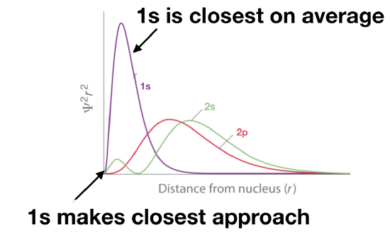
1. Which of the orbitals in Figure \(\PageIndex{1}\) is closest to the nucleus?

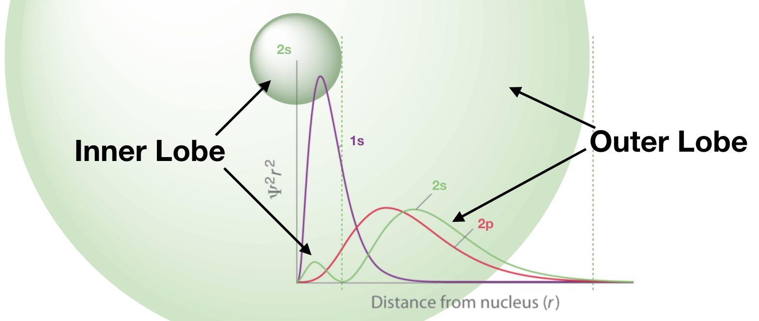
2. Explain why the plot of the 2s orbital has two humps?

3. What is represented by the vertical dashed lines in Figure \(\PageIndex{1}\)?

4. Why does the 2p orbital have only one hump?

Answer 1

The 1s orbital: Not only does its probability function make the closest approach to the nucleus, it is also on average closer than 2s or 2p.

.

Answer 2

The 2s has two lobes, each is represented by a unique hump in the radial probability function.

Answer 3

These lines represent boundary surfaces and nodes that define the shape and boundaries of the orbital. Most of the vertical dashed lines represent boundary surfaces (where the function approaches zero at far distances from the nucleus). Only the 2s orbital has a radial node that is represented by the vertical dashed line between its two nodes.

Answer 4

The 2p orbital has two lobes (similar to 2s) and so you might expect it to have two humps. However, the radial probability functions are expressed only in one direction; there is no negative value for the radius! The radial probability function of the p orbital would look the same in either direction, as long as the axis of the plot is colinear with the orbital's axis.

Further Reading

If you'd like to understand more about what the Schrödinger equation is and where the orbital shapes and/or the radial probability functions come from, read the pages in section 2.2 of the Inorganic Chemistry Textmap here (click): I've written them to be appropriate for inorganic chemistry students who have not yet had P-Chem.