5.2: Jupyter Notebooks (Executable Programming Code and Figures)
- Page ID
- 211889
\( \newcommand{\vecs}[1]{\overset { \scriptstyle \rightharpoonup} {\mathbf{#1}} } \)
\( \newcommand{\vecd}[1]{\overset{-\!-\!\rightharpoonup}{\vphantom{a}\smash {#1}}} \)
\( \newcommand{\id}{\mathrm{id}}\) \( \newcommand{\Span}{\mathrm{span}}\)
( \newcommand{\kernel}{\mathrm{null}\,}\) \( \newcommand{\range}{\mathrm{range}\,}\)
\( \newcommand{\RealPart}{\mathrm{Re}}\) \( \newcommand{\ImaginaryPart}{\mathrm{Im}}\)
\( \newcommand{\Argument}{\mathrm{Arg}}\) \( \newcommand{\norm}[1]{\| #1 \|}\)
\( \newcommand{\inner}[2]{\langle #1, #2 \rangle}\)
\( \newcommand{\Span}{\mathrm{span}}\)
\( \newcommand{\id}{\mathrm{id}}\)
\( \newcommand{\Span}{\mathrm{span}}\)
\( \newcommand{\kernel}{\mathrm{null}\,}\)
\( \newcommand{\range}{\mathrm{range}\,}\)
\( \newcommand{\RealPart}{\mathrm{Re}}\)
\( \newcommand{\ImaginaryPart}{\mathrm{Im}}\)
\( \newcommand{\Argument}{\mathrm{Arg}}\)
\( \newcommand{\norm}[1]{\| #1 \|}\)
\( \newcommand{\inner}[2]{\langle #1, #2 \rangle}\)
\( \newcommand{\Span}{\mathrm{span}}\) \( \newcommand{\AA}{\unicode[.8,0]{x212B}}\)
\( \newcommand{\vectorA}[1]{\vec{#1}} % arrow\)
\( \newcommand{\vectorAt}[1]{\vec{\text{#1}}} % arrow\)
\( \newcommand{\vectorB}[1]{\overset { \scriptstyle \rightharpoonup} {\mathbf{#1}} } \)
\( \newcommand{\vectorC}[1]{\textbf{#1}} \)
\( \newcommand{\vectorD}[1]{\overrightarrow{#1}} \)
\( \newcommand{\vectorDt}[1]{\overrightarrow{\text{#1}}} \)
\( \newcommand{\vectE}[1]{\overset{-\!-\!\rightharpoonup}{\vphantom{a}\smash{\mathbf {#1}}}} \)
\( \newcommand{\vecs}[1]{\overset { \scriptstyle \rightharpoonup} {\mathbf{#1}} } \)
\( \newcommand{\vecd}[1]{\overset{-\!-\!\rightharpoonup}{\vphantom{a}\smash {#1}}} \)
\(\newcommand{\avec}{\mathbf a}\) \(\newcommand{\bvec}{\mathbf b}\) \(\newcommand{\cvec}{\mathbf c}\) \(\newcommand{\dvec}{\mathbf d}\) \(\newcommand{\dtil}{\widetilde{\mathbf d}}\) \(\newcommand{\evec}{\mathbf e}\) \(\newcommand{\fvec}{\mathbf f}\) \(\newcommand{\nvec}{\mathbf n}\) \(\newcommand{\pvec}{\mathbf p}\) \(\newcommand{\qvec}{\mathbf q}\) \(\newcommand{\svec}{\mathbf s}\) \(\newcommand{\tvec}{\mathbf t}\) \(\newcommand{\uvec}{\mathbf u}\) \(\newcommand{\vvec}{\mathbf v}\) \(\newcommand{\wvec}{\mathbf w}\) \(\newcommand{\xvec}{\mathbf x}\) \(\newcommand{\yvec}{\mathbf y}\) \(\newcommand{\zvec}{\mathbf z}\) \(\newcommand{\rvec}{\mathbf r}\) \(\newcommand{\mvec}{\mathbf m}\) \(\newcommand{\zerovec}{\mathbf 0}\) \(\newcommand{\onevec}{\mathbf 1}\) \(\newcommand{\real}{\mathbb R}\) \(\newcommand{\twovec}[2]{\left[\begin{array}{r}#1 \\ #2 \end{array}\right]}\) \(\newcommand{\ctwovec}[2]{\left[\begin{array}{c}#1 \\ #2 \end{array}\right]}\) \(\newcommand{\threevec}[3]{\left[\begin{array}{r}#1 \\ #2 \\ #3 \end{array}\right]}\) \(\newcommand{\cthreevec}[3]{\left[\begin{array}{c}#1 \\ #2 \\ #3 \end{array}\right]}\) \(\newcommand{\fourvec}[4]{\left[\begin{array}{r}#1 \\ #2 \\ #3 \\ #4 \end{array}\right]}\) \(\newcommand{\cfourvec}[4]{\left[\begin{array}{c}#1 \\ #2 \\ #3 \\ #4 \end{array}\right]}\) \(\newcommand{\fivevec}[5]{\left[\begin{array}{r}#1 \\ #2 \\ #3 \\ #4 \\ #5 \\ \end{array}\right]}\) \(\newcommand{\cfivevec}[5]{\left[\begin{array}{c}#1 \\ #2 \\ #3 \\ #4 \\ #5 \\ \end{array}\right]}\) \(\newcommand{\mattwo}[4]{\left[\begin{array}{rr}#1 \amp #2 \\ #3 \amp #4 \\ \end{array}\right]}\) \(\newcommand{\laspan}[1]{\text{Span}\{#1\}}\) \(\newcommand{\bcal}{\cal B}\) \(\newcommand{\ccal}{\cal C}\) \(\newcommand{\scal}{\cal S}\) \(\newcommand{\wcal}{\cal W}\) \(\newcommand{\ecal}{\cal E}\) \(\newcommand{\coords}[2]{\left\{#1\right\}_{#2}}\) \(\newcommand{\gray}[1]{\color{gray}{#1}}\) \(\newcommand{\lgray}[1]{\color{lightgray}{#1}}\) \(\newcommand{\rank}{\operatorname{rank}}\) \(\newcommand{\row}{\text{Row}}\) \(\newcommand{\col}{\text{Col}}\) \(\renewcommand{\row}{\text{Row}}\) \(\newcommand{\nul}{\text{Nul}}\) \(\newcommand{\var}{\text{Var}}\) \(\newcommand{\corr}{\text{corr}}\) \(\newcommand{\len}[1]{\left|#1\right|}\) \(\newcommand{\bbar}{\overline{\bvec}}\) \(\newcommand{\bhat}{\widehat{\bvec}}\) \(\newcommand{\bperp}{\bvec^\perp}\) \(\newcommand{\xhat}{\widehat{\xvec}}\) \(\newcommand{\vhat}{\widehat{\vvec}}\) \(\newcommand{\uhat}{\widehat{\uvec}}\) \(\newcommand{\what}{\widehat{\wvec}}\) \(\newcommand{\Sighat}{\widehat{\Sigma}}\) \(\newcommand{\lt}{<}\) \(\newcommand{\gt}{>}\) \(\newcommand{\amp}{&}\) \(\definecolor{fillinmathshade}{gray}{0.9}\)CKEditor is a rich text editor which enables the user to write content directly inside web pages or online applications. Through the Binder Plugin, authors of textbooks have the option to include code within their textbook pages to create a more interactive experience for their students. Currently the plugin supports Python 3, Julia, R, Octave, C++, and SageMath. Additionally, all languages with the exception of SageMath support syntax highlighting for an easier scripting experience.
The following video tutorial provides a step-by-step walkthrough of the tutorial.
Step-by-Step Process to use CKEditor Binder Plugin
Creating a new page
Authors have the option to add code to a new page.

Editing an existing page
Additionally, authors can also add code to pages that they have already created. To do so, simply click on the "Edit" button.

Locating the Plugin and Adding Code
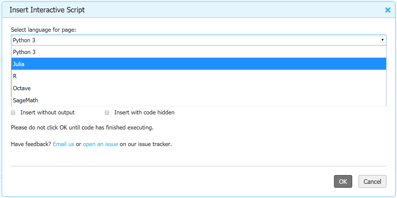
The Binder Logo is the last button on the navigation bar of the text editor. Binder is an external resource that lets you build and run kernels which contain the necessary packages for executing any given code language.

Add Code
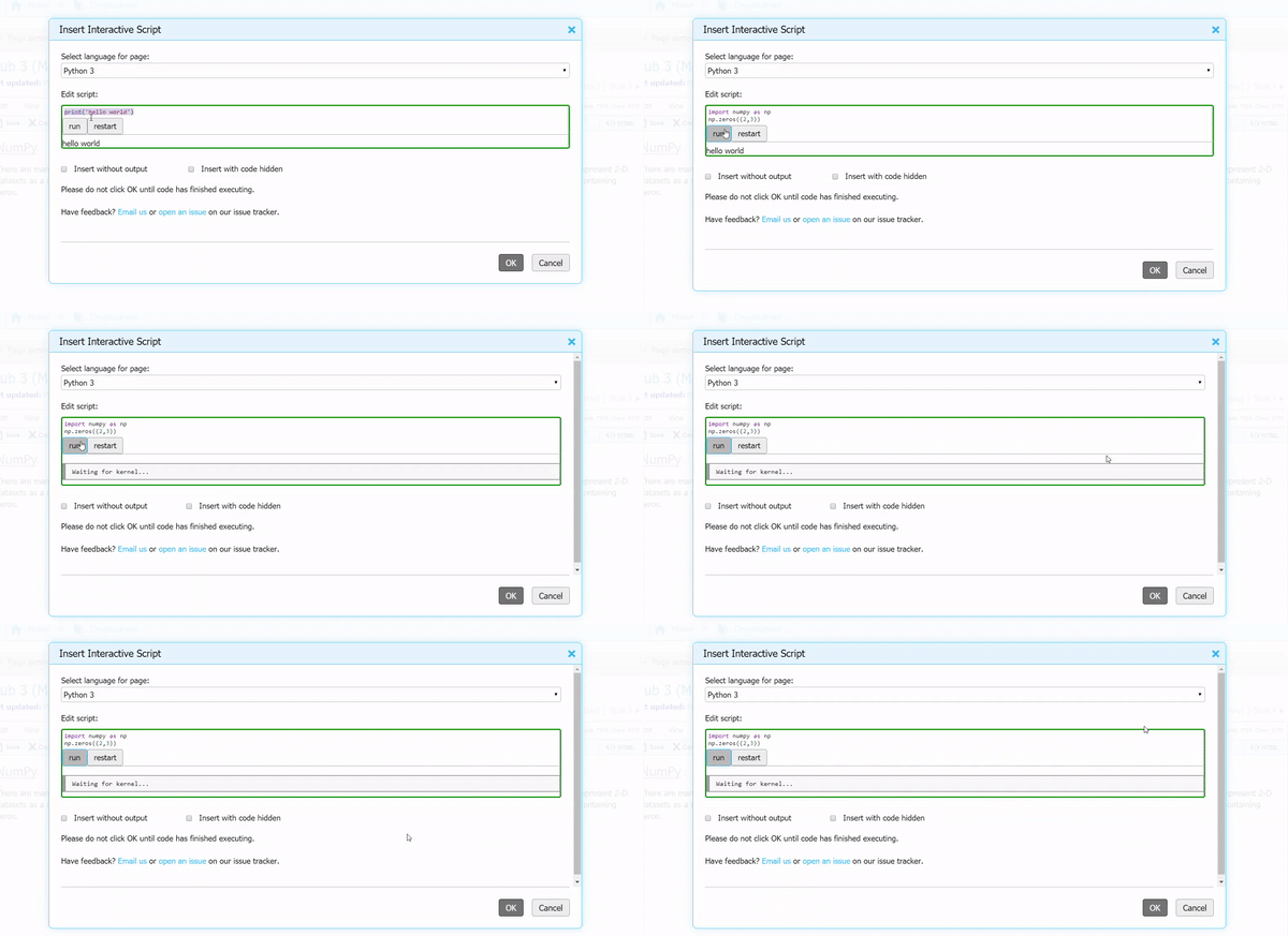
To add a block of code, select the language and add your code in the text space. Be sure to press "run" and verify the code output before inserting the code cell into your page. This output will be displayed by default on the webpage even if the cell has not been run by the reader.
Add Data
Step 1:
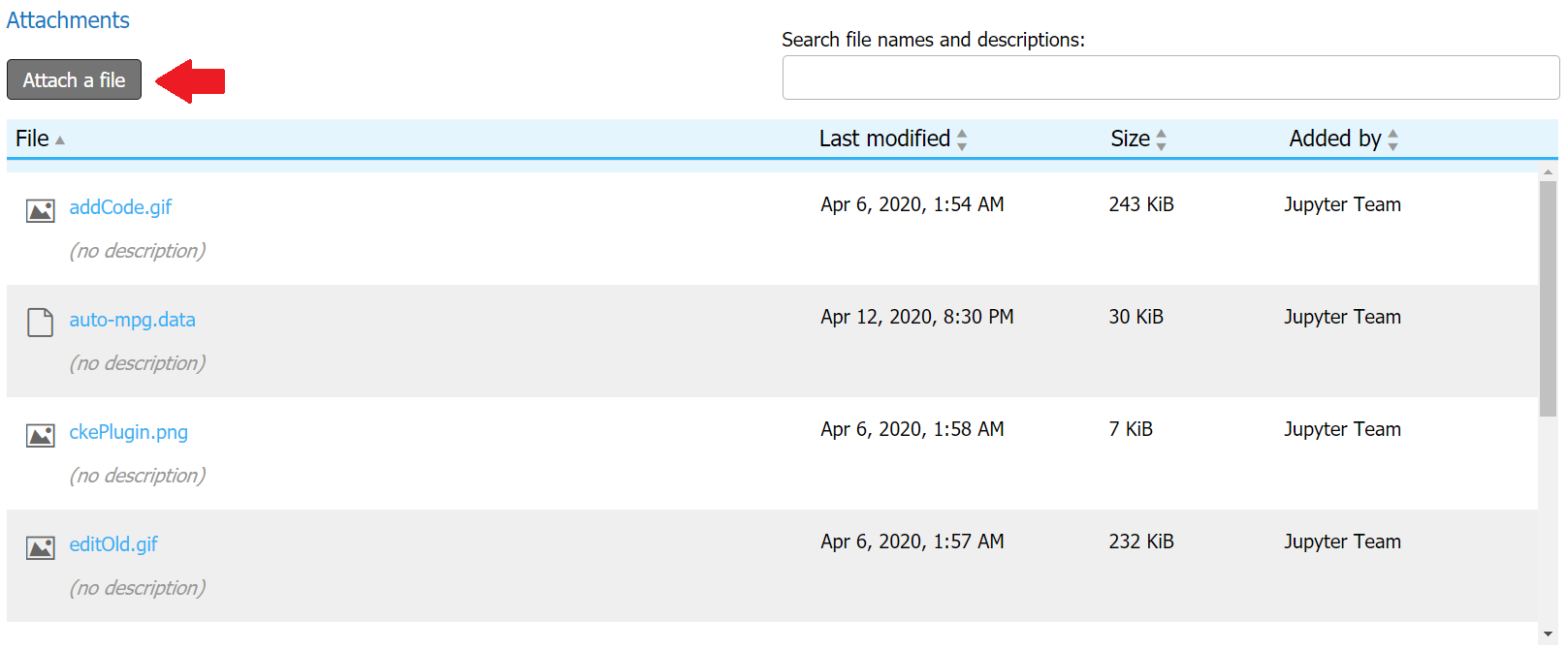
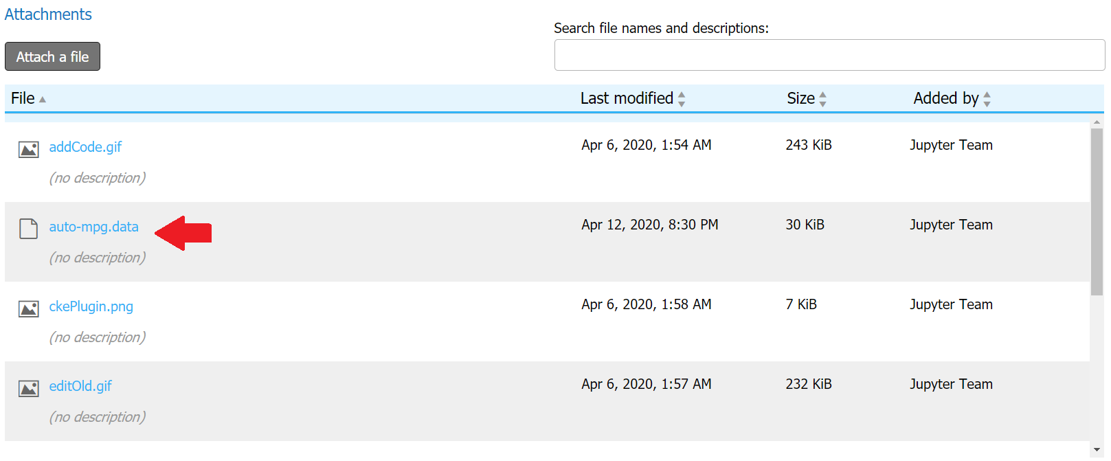
Go to the bottom of the page and attach data file by clicking "Attach a file" link.
Step 2:
Select the file you want to upload from your local computer, and attach file.
Step 3:
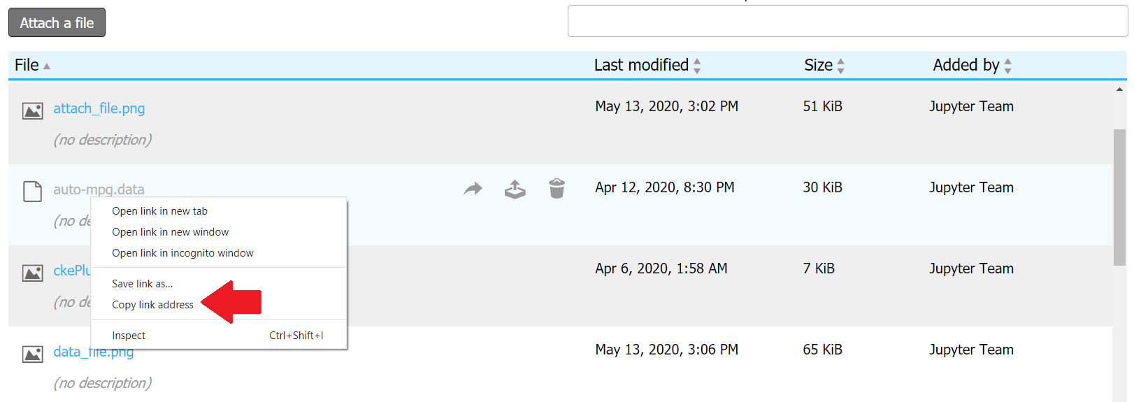
Right click and get link address of file you have uploaded.
Step 4:
To incorporate data into code, click CKEditor Binder Button, select language, and follow the examples below respective to the language you have chosen. when following the tutorial, replace the URL in the example with the one you have.
For Python 3:
This page provides multiples ways to incorporate data into your code blocks, and some possible examples of what you may want to do with your code.
For R:
This tutorial goes over some ways in which to load a data file from a URL for R
For Julia:
View this page to load a file from an URL in Julia
For C++:
Here are some ways for C++.
For SageMath:
This tutorial goes over some ways in which to load a data file from a URL for SageMath
For Octave:
View this page for Octave.
An Example Page
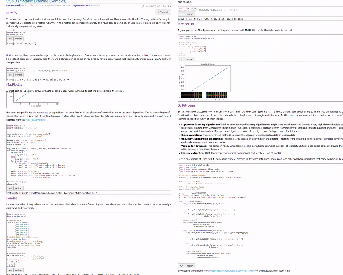
Remember to press save once edits to the page are done, the following is an example page utilizing the Binder Plugin. As seen, authors can use libraries and packages already available. If a package you would like to use is not available, simply email us, or open an issue on the GitHub repository (information found in the dialogue box of the plugin).
How does CKEditor Binder Plugin Work? (Work in Progress)
A Jupyter Notebook Backend
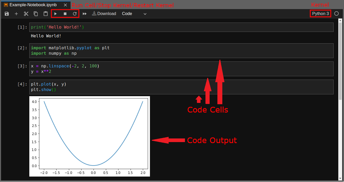
As mentioned above, CKEditor is the general interface that you use to edit Libretexts pages, while the CKEdtitor Binder plugin allows you to insert code cells and is accessed via the navigation bar in the text editor. The best way to understand how the Binder plugin works is to think of it as turning your Libretexts page into a Jupyter notebook. As explained by Jupyter, these notebooks "are both human-readable documents containing the analysis description and the results [of some project] (figures, tables, etc..) as well as executable documents which can be run to perform data analysis". This means that they can contain both computer code and rich text elements. Put this way it becomes clear as to how a Libretexts page, which may contain richly styled text in addition to code cells, operates very similarly to a Jupyter notebook.
Just like in Jupyter notebooks, the Binder plugin uses kernels to execute code cells. On Libretexts, when you insert an interactive script and select a language the plugin will provide you with the proper kernel to execute that language. Each page may have only one kernel (programming language), and the kernel is activated behind the scenes the first time you "run" a code cell on a page. Once activated, the kernel remains alive and activated across the entire webpage just as it would in a Jupyter notebook. For instance, this is why you can put all of your Python importstatements into a single code cell at the beginning of your document and later make calls to those modules in seperate cells.
The Jupyter notebook image below should help solidify the analogy even further.
