10.3.1: Intrinsic and Extrinsic Fluorophores

Intrinsic and Extrinsic Fluorophores

An intrinsic fluorophore is a ion, molecule or macromolecule that fluoresces strongly in it native form while an extrinsic fluorophore is a species that has been made to fluoresce strongly through reaction with a fluorometric reagent.

Among organic molecules only a small fraction are intrinsic fluorophores.  These molecules tend to possess rigid structures, that hinder release of the excited state energy to the bath, and extensive delocalized \(pi\) bonding networks.  Fluorescein and quinine are good examples of fluorophores with large quantum yields.

 

Figure \(\PageIndex{1}\): The structures of fluorescein and quinine.

Both the quantum yield and the emission wavelength can change for fluorophores that can participate in acid base chemistry depending on whether they are protonated or not.

Most metal ions, be they main group ions, transition metal ions do not fluoresce and only a few lanthanide ions fluoresce weakly.  In fact metal ions that are paramagnetic are more likely phosphoresce following intersystem crossing or to act to quench the fluorescence of an excited state fluorophore.  Also for transition metal ions, they are characterized by many closely spaced energy levels which increases the likelihood of deactivation by internal conversion. 

Extrinsic fluorophores can be formed via chelation reactions with many metal ions.  A metal chelate is a combination of a metal ion with an organic molecule to which the metal ion is attached at one point by a primary bond and to another part of the molecule by a secondary bond.  Common linkages are from between a metal ion with a 2,2'-dihydroxy azo dye  or 8-quinolinol and are shown below in Figure\(\PageIndex{2}\): for (1) Al and (2) Be.

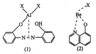
Figure \(\PageIndex{2}\): Two examples of metal chelate structures

This combination usually results in the metal ion being a member of a 5 or 6 membered ring, increasing the rigidity of the organic molecule.  This combination is not the cause or origin of the fluorescence because the molecule is likely to be weakly fluorescent.  However, in many cases the emission is shifted to a longer wavelength and the fluorescence intensity is greatly increased.

For the lanthanides ion, the fluorescence of the metal chelate complexes is most intense when the metal ion has the oxidation state of of 3+. Not all lanthanide metals can be used and the most common are: Sm(III), Eu(III), Tb(III), and Dy(III)

In the realm of biochemistry and bioanalytical chemistry, tryptophan is the only intrinsic fluorophore among the natural amino acids and it's excitation and emission wavelengths are in the UV (maximum absorption of 280 nm and an emission peak that is solvatochromic, ranging from 300 to 350 nm depending in the polarity of the local environment).  DNA and RNA are not intrinsic fluorophores.

Proteins, DNA and RNA can be made fluorescent thorough well established labeling chemistry with fluormetric reagents that are either reactive towards amines and carboxylic acids or in the case of DNA, intercalate between the base pairs.   Two example of fluorometric reagents that react with amines are show in Figure\(\PageIndex{3}\): below.   

Figure \(\PageIndex{3}\): Two fluorometric reagents used to put a fluorescent label on a biological macromolecule through a reaction with an amine group.

One of the most important developments in bioanalytical chemistry has been the development and application of the green fluorescent protein first isolated from jelly fish in the 1960's and 1970's .  The original close of the green fluorescent protein were not particularly useful due to dual peaked excitation spectra, pH sensitivity, chloride sensitivity, poor fluorescence quantum yield, poor photostability and poor folding at 37 °C.  However, due to the potential for widespread usage and the evolving needs of researchers, many different mutants of GFP have been engineered.  The first major improvement was a single point mutation (S65T) reported in 1995 in Nature by Roger Tsien.  This mutation dramatically improved the spectral characteristics of GFP, resulting in increased fluorescence, photostability, and a shift of the major excitation peak to 488 nm, with the peak emission kept at 509 nm. As shown in Figure \(\PageIndex{4}\): below, many other mutations are available, including different color mutants; in particular, blue fluorescent protein, cyan fluorescent protein, and yellow fluorescent protein derivatives.

Figure \(\PageIndex{4}\): "Imaging Life with Fluorescent Proteins" by ZEISS Microscopy is licensed under CC BY-SA 2.0