5.3: The Harmonic Oscillator Approximates Vibrations

The quantum harmonic oscillator is the quantum analog of the classical harmonic oscillator and is one of the most important model systems in quantum mechanics. This is due in partially to the fact that an arbitrary potential curve \(V(x)\) can usually be approximated as a harmonic potential at the vicinity of a stable equilibrium point. Furthermore, it is one of the few quantum-mechanical systems for which an exact, analytical solution exists. Solving other potentials typically require either approximations or numerical approaches to identify the corresponding eigenstates and eigenvalues (i.e., wavefunctions and energies).

Figure \(\PageIndex{1}\): The \(\ce{HCl}\) molecule is really an anharmonic oscillator. Here \(HCl\) is vibrating at energy level \(E_3\). \(D_0\) is dissociation energy here, \(r_0\) bond length, \(V\) potential energy. Energy is expressed in wavenumbers. The hydrogen chloride molecule is attached to the coordinate system to show bond length changes on the curve. from Wikipedia.

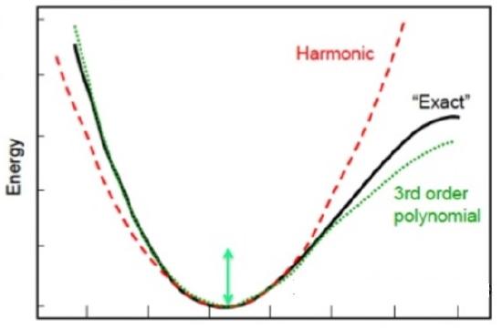
A general potential energy (\(V(x)\)) curve for a molecular vibration can be expanded as a Taylor series (Figure \(\PageIndex{2}\))

\[V(x) = V(x_0) + \left. \dfrac {d V(x)}{d x} \right|_{x_0}^{x} (x - x_0) + \left. \dfrac {1}{2!} \dfrac {d^2 V(x)}{d x^2} \right|_{x_0}^{x} (x - x_0)^2 + \ldots + \left. \dfrac {1}{n!} \dfrac {d^n V(x)}{d x^n} \right|_{x_0}^{x} (x - x_0)^n \label{5.3.1}\]

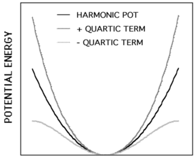
\(V(x)\) is often (but not always) shortened to the cubic term and can be rewritten as

\[V(x) = \dfrac {1}{2} kx^2 + \dfrac {1}{6} \gamma x^3 \label{5.3.2}\]

where \(V(x_0) = 0\), \(k\) is the harmonic force constant (harmonic term), and \(\gamma\) is the first (i.e., cubic) anharmonic term. It is important to note that this approximation is only good for \(x\) near \(x_0\), and that \(x_0\) stands for the equilibrium bond distance.

Figure \(\PageIndex{2}\): (left) Deviation from simple harmonic potential approximation (red curve) of true/exact potential (black curve) with cubic term (green). (right) Expansion with positive or negative quartic terms. Images used with permission from Heather Kulik (MIT) via OpenCourseWare.

Almost all diatomics have experimentally determined \(\dfrac {d^2 V}{d x^2}\) for their lowest energy states. H₂, Li₂, O₂, N₂, and F₂ have had terms up to \(n < 10\) determined of Equation \(\ref{5.3.1}\).

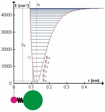
Adding anharmonic perturbations to the harmonic oscillator (Equation \(\ref{5.3.2}\)) better describes molecular vibrations. Anharmonic oscillation is defined as the deviation of a system from harmonic oscillation, or an oscillator not oscillating in simple harmonic motion. Anharmonic oscillation is described as the restoring force is no longer proportional to the displacement. Figure \(\PageIndex{1}\) shows the the general potential with (numerically) calculated energy levels (\(E_0\), \(E_1\) etc.). \(D_o\) is the dissociation energy, which is different from the well depth \(D_e\). These vibrational energy levels of this plot can be calculated using the harmonic oscillator model (i.e., Equation \(\PageIndex{1}\) with the Schrödinger equation) and have the general form

\[ E_v = \left(v + \dfrac{1}{2}\right) v_e - \left(v + \dfrac{1}{2}\right)^2 v_e x_e + \left(v + \dfrac{1}{2}\right)^3 v_e y_e + \text{higher terms} \label{5.3.7}\]

where \( v \) is the vibrational quantum number and \( x_e\) and \( y_e\) are the first and second anharmonicity constants, respectively.

The \(v = 0\) level is the vibrational ground state. Because this potential is less confining than a parabola used in the harmonic oscillator, the energy levels become less widely spaced at high excitation (Figure \(\PageIndex{1}\); top of potential).

Limitations of the Harmonic Oscillator Model for Molecular Vibrations

The harmonic oscillation is a great approximation of a molecular vibration, but has key limitations:

• Due to equal spacing of energy, all transitions occur at the same frequency (i.e. single line spectrum). However experimentally many lines are often observed (called overtones).
• The harmonic oscillator does not predict bond dissociation; you cannot break it no matter how much energy is introduced.

Morse Potentials are better Approximations of Vibrational Motion

A more powerful approach than just "patching up" the harmonic oscillator solution with anharmonic corrections is to adopt a different potential (\(V(x)\)). One such approach is the Morse potential, named after physicist Philip M. Morse, and a better approximation for the vibrational structure of the molecule than the harmonic oscillator because it explicitly includes the effects of bond breaking and accounts for the anharmonicity of real bonds (Figure \(\PageIndex{4}\)).

Figure \(\PageIndex{4}\): The Morse potential (blue) and harmonic oscillator potential (green). Unlike the energy levels of the harmonic oscillator potential, which are evenly spaced by ħω, the Morse potential level spacing decreases as the energy approaches the dissociation energy. The dissociation energy \(D_e\) is larger than the true energy required for dissociation \(D_0\) due to the zero point energy of the lowest (\(v = 0\)) vibrational level. from Wikipedia.

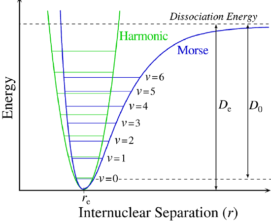
The Morse Potential is a good approximation to \(V(x)\) and is best when looking for a general formula for all \(x\) from 0 to \(\infty\), not just applicable for the local region around the \(x_o\):

\[V(x) = D(1-e^{-\beta (x - x_0)})^2 \label{5.3.8}\]

with \(V(x = x_0) = 0\) and \(V(x = \infty) = D\).

The Morse Potential (Figure \(\PageIndex{4}\)) approaches zero at infinite \(r_e\) and equals \(-D_e\) at its minimum (i.e. \(r=r_e\)). It clearly shows that the Morse potential is the combination of a short-range repulsion term (small \(r\) values) and a long-range attractive term (large \(r\) values).

Solving the Schrödinger Equation with the Morse Potential (Equation \ref{5.3.8}) is not trivial, but can be done analytically.

\[ \hat{H}|\psi \rangle = E_n | \psi \rangle \]

with

\[ \begin{align} \hat{H} &= \hat{T} + \hat{V} \\[4pt] &= \dfrac{- \hbar ^2 d^2}{2m \;dx^2} + D(1-e^{-\beta (x - x_0)})^2 \label{5.3.9} \end{align} \]

The solutions and energies for the Morse potential will not be used in this course and will not be discussed in more detail.

Contributors

• Peter Kelly (UCDavis)