5.4: The Harmonic Oscillator Energy Levels

For a classical oscillator, we know exactly the position, velocity, and momentum as a function of time. The frequency of the oscillator (or normal mode) is determined by the reduced mass \(\mu\) and the effective force constant \(k\) of the oscillating system and does not change unless one of these quantities is changed. There are no restrictions on the energy of the oscillator, and changes in the energy of the oscillator produce changes in the amplitude of the vibrations experienced by the oscillator.

Figure \(\PageIndex{1}\): Potential energy function and first few energy levels for harmonic oscillator.

For the quantum mechanical oscillator, the oscillation frequency of a given normal mode is still controlled by the mass and the force constant (or, equivalently, by the associated potential energy function). However, the energy of the oscillator is limited to certain values. The allowed quantized energy levels are equally spaced and are related to the oscillator frequencies as given by Equation \(\ref{5.4.1}\) and Figure \(\PageIndex{1}\).

\[E_v = \left ( v + \dfrac {1}{2} \right ) \hbar \omega = \left ( v + \dfrac {1}{2} \right ) h \nu \label {5.4.1}\]

with

\[v = 0, 1, 2, 3, \cdots \infty \]

In a quantum mechanical oscillator, we cannot specify the position of the oscillator (the exact displacement from the equilibrium position) or its velocity as a function of time; we can only talk about the probability of the oscillator being displaced from equilibrium by a certain amount. This probability is given by

\[P_{Q \rightarrow Q + dQ} = \int_{Q}^{Q + dQ} \psi ^*_v (Q) \psi _v (Q) dQ \label {5.4.3}\]

We can, however, calculate the average displacement and the mean square displacement of the atoms relative to their equilibrium positions. This average is just \(\left \langle Q \right \rangle\), the expectation value for \(Q\), and the mean square displacement is \(\left \langle Q^2 \right \rangle\), the expectation value for \(Q^2\). Similarly we can calculate the average momentum \(\left \langle P_Q \right \rangle\), and the mean square momentum \(\left \langle P^2_Q \right \rangle\), but we cannot specify the momentum as a function of time.

Physically what do we expect to find for the average displacement and the average momentum? Since the potential energy function is symmetric around \(Q = 0\), we expect values of \(Q > 0\) to be equally as likely as \(Q < 0\). The average value of \(Q\) therefore should be zero.

These results for the average displacement and average momentum do not mean that the harmonic oscillator is sitting still. As for the particle-in-a-box case, we can imagine the quantum mechanical harmonic oscillator as moving back and forth and therefore having an average momentum of zero. Since the lowest allowed harmonic oscillator energy, \(E_0\), is \(\dfrac{\hbar \omega}{2}\) and not 0, the atoms in a molecule must be moving even in the lowest vibrational energy state. This phenomenon is called the zero-point energy or the zero-point motion, and it stands in direct contrast to the classical picture of a vibrating molecule. Classically, the lowest energy available to an oscillator is zero, which means the momentum also is zero, and the oscillator is not moving.

Exercise \(\PageIndex{1}\)

Compare the quantum mechanical harmonic oscillator to the classical harmonic oscillator at \(v=1\) and \(v=50\).

Answer

At v=1 the classical harmonic oscillator poorly predicts the results of quantum mechanical harmonic oscillator, and therefore reality. At v=1 the particle will be near the ground state and the classical model will predict the particle to spend most it's time on the outer edges when the KE goes to zero and PE is at a maximum, while the quantum model says the opposite and that the particle will be more likely to be found in the center. At v=50 the quantum model will begin to match the classical much more closely, with the particle most likely to be found at the edges. The quantum model looking more like the classical at higher quantum numbers can be referred to as the correspondence principle.

Since the average values of the displacement and momentum are all zero and do not facilitate comparisons among the various normal modes and energy levels, we need to find other quantities that can be used for this purpose. We can use the root mean square deviation (see also root-mean-square displacement) (also known as the standard deviation of the displacement) and the root-mean-square momentum as measures of the uncertainty in the oscillator's position and momentum.

For a molecular vibration, these quantities represent the standard deviation in the bond length and the standard deviation in the momentum of the atoms from the average values of zero, so they provide us with a measure of the relative displacement and the momentum associated with each normal mode in all its allowed energy levels. These are important quantities to determine because vibrational excitation changes the size and symmetry (or shape) of molecules. Such changes affect chemical reactivity, the absorption and emission of radiation, and the dissipation of energy in radiationless transitions.

The harmonic oscillator wavefunctions form an orthonormal set; this means that all functions in the set are normalized individually

\[\int \limits _{-\infty}^{\infty} \psi ^*_v (x) \psi _v (x) dx = 1 \label {5.4.4}\]

and are orthogonal to each other.

\[\int \limits _{-\infty}^{\infty} \psi ^*_{v'} (x) \psi _v (x) dx = 0 \;\; \text {for} \;\; v' \ne v \label {5.4.5}\]

The fact that a family of wavefunctions forms an orthonormal set is often helpful in simplifying complicated integrals. We will use these properties when we determine the harmonic oscillator selection rules for vibrational transitions in a molecule and calculate the absorption coefficients for the absorption of infrared radiation.

Finally, we can calculate the probability that a harmonic oscillator is in the classically forbidden region. What does this tantalizing statement mean? Classically, the maximum extension of an oscillator is obtained by equating the total energy of the oscillator to the potential energy, because at the maximum extension all the energy is in the form of potential energy. If all the energy weren't in the form of potential energy at this point, the oscillator would have kinetic energy and momentum and could continue to extend further away from its rest position. Interestingly, as we show below, the wavefunctions of the quantum mechanical oscillator extend beyond the classical limit, i.e. beyond where the particle can be according to classical mechanics.

The lowest allowed energy for the quantum mechanical oscillator is called the zero-point energy, \(E_0 = \dfrac {\hbar \omega}{2} \). Using the classical picture described in the preceding paragraph, this total energy must equal the potential energy of the oscillator at its maximum extension. We define this classical limit of the amplitude of the oscillator displacement as \(Q_0\). When we equate the zero-point energy for a particular normal mode to the potential energy of the oscillator in that normal mode, we obtain

\[ \dfrac {\hbar \omega}{2} = \dfrac {k Q^2_0}{2} \label {5.4.6}\]

The zero-point energy is the lowest possible energy that a quantum mechanical physical system may have. Hence, it is the energy of its ground state.

Recall that \(k\) is the effective force constant of the oscillator in a particular normal mode and that the frequency of the normal mode is given by Equation \(\ref{5.4.1}\) which is

\[\omega = \sqrt {\dfrac {k}{\mu}} \label {5.4.7}\]

Example \(\PageIndex{2}\): Hydrogen Chloride

The \(\ce{HCl}\) equilibrium bond length is 0.127 nm and the \(v = 0\) to \(v = 1\) transition is observed in the infrared at 2,886 cm^-1. Compute the vibrational energy of HCl in its lowest state. Compute the classical limit for the stretching of the \(\ce{HCl}\) bond from its equilibrium length in this state. What percent of the equilibrium bond length is this extension?

Solution

H-Cl bond length = 0.127nm = 1.27 * 10^-10m

Transition observed at 2886 cm^-1 => 2886 cm^-1 * (3*10^10 cm/s) = 8.646*10^13 s^-1 or 8.656*10^13 Hz

E_v = (v + 1/2)(hbar)(w), or, at v=0 (ground state), E₀ = (1/2)(hbar)(w)

The term w (omega) is equal to sqrt(k/u) where k is the force constant of the molecular bond and u is the reduced mass of the molecule.

Reduced mass = m1m2/(m1+m2) or ~ (17)(1)/(17+1) amu

or when converted into kg, is 1.568*10^-27kg

The term w is also equal to 2(pi)(f), so we can solve for k by the equality 2(pi)(f) = sqrt(k/u) or

2(pi)(8.656*10^-13 Hz) = sqrt(k/(1.57*10^-27 kg)) where we obtain k = 481 N/m

and w = sqrt((481 N/m)/1.57*10^27 kg)) = 5.54*10^14 rad/s

We can then acquire the ground state vibrational energy from

E₀ = (1/2)(hbar)(w) = (1/2)(hbar)(5/54*10^14 rad/s) = 2.916*10^-20 J

The classical limit of the stretch is denoted as Q₀, this can be equated as potential energy in relation to the total E₀ found above as, at E₀, all of the energy would be potential energy in the form of the stretch. In comparison to the classic spring force equation, Q₀ is calculated as V = (1/2)(k)(Q₀^2)

As described above, we can relate the two as (1/2)(hbar)(w) = (1/2)(k)(Q₀^2)

or, 2.916*10^-20 J = (1/2)(481)(Q₀^2) where Q₀ = 1.10*10^-11 m or 0.0110 nm

Lastly, this classical limit to length can be compared to the equilibrium bond length by a simple relation of

(Q₀/x_eq)*100 = Percent bond length => (0.110nm)/(0.127nm)*100 = 8.66%

Examination of the quantum mechanical wavefunction for the lowest-energy state reveals that the wavefunction \(Ψ_0(x)\) extends beyond the classical limit (i.e., outside of the harmonic oscillator well, albeit slightly). Higher energy states have higher total energies, so the classical limits to the amplitude of the displacement will be larger for these states.

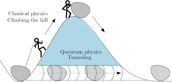
Tunneling

The observation that the wavefunctions are not zero at the classical limit means that the quantum mechanical oscillator has a finite probability of having a displacement that is larger than what is classically possible. The oscillator can be in a region of space where the potential energy is greater than the total energy. Classically, when the potential energy equals the total energy, the kinetic energy and the velocity are zero, and the oscillator cannot pass this point. A quantum mechanical oscillator, however, has a finite probability of passing this point. For a molecular vibration, this property means that the amplitude of the vibration is larger than what it would be in a classical picture. In some situations, a larger amplitude vibration could enhance the chemical reactivity of a molecule.

Figure \(\PageIndex{2}\): In classical mechanics a particle can only pass through a barrier if it has enough kinetic energy to get over the barrier in potential energy. A quantum particle can sometimes sneak through a barrier even when its energy would seem to trap it on one side. This effect, called quantum tunneling, explains how trapped nuclear particles can sometimes escape their nuclei, leading to radioactive decay. Tunneling also allows photons of visible light to escape the interior of the sun and electrical currents to function.

Exercise \(\PageIndex{3}\)

Plot the probability density for \(v = 0\) and \(v = 1\) states. Mark the classical limits on each of the plots, since the limits are different because the total energy is different for \(v = 0\) and \(v = 1\). Shade in the regions of the probability densities that extend beyond the classical limit.

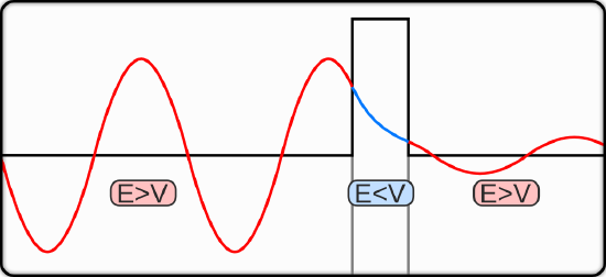
The fact that a quantum mechanical oscillator has a finite probability to enter the classically forbidden region of space is a consequence of the wave property of matter and the Heisenberg Uncertainty Principle. A wave changes gradually, and the wavefunction approaches zero gradually as the potential energy approaches infinity.

To understand quantum tunneling, think about a particle moving on a line. Now imagine placing a wall on each side of the particle. In classical physics, the particle bounces back and forth between the walls and eventually stops, trapped. The particle has enough energy to be outside the walls, but it does not have enough energy to get there.

Figure \(\PageIndex{2}\): (left) Classical behavior of a particle colliding with a barrier of finite thickness and height. (right) Corresponding quantum behavior. This chance to be found beyond the barrier is called the tunneling probability.

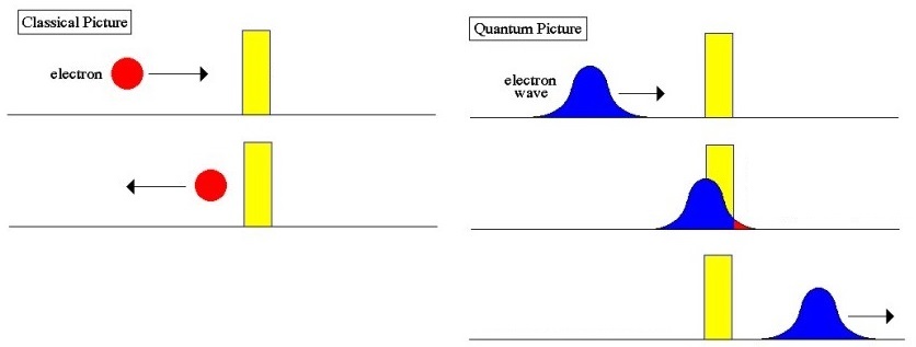
In quantum mechanics, the particle behaves like a wave. The wave is most intense between the walls, so the particle is probably there. At the walls, the quantum wave diminishes but does not become zero; it extends slightly into the walls. A very low-intensity wave extends outside the walls. There is thus a tiny probability that the particle will be found outside the walls.

Figure \(\PageIndex{3}\): Quantum tunnelling through a barrier. The energy of the tunneled particle is the same but the probability amplitude is decreased. (CC-SA-BY 3.0; Felix Kling).

Tunneling in Harmonic Oscillators

We should be able to calculate the probability that the quantum mechanical harmonic oscillator is in the classically forbidden region for the lowest energy state of the harmonic oscillator, the state with \(v = 0\). The classically forbidden region is shown by the shading of the regions beyond \(Q_0\) in the graph you constructed for Exercise \(\PageIndex{3}\). The area of this shaded region gives the probability that the bond oscillation will extend into the forbidden region (Figure \(\PageIndex{3}\)). To calculate this probability, we use

\[ P [ \text {forbidden}] = 1 - P [ \text {allowed}] \label {5.4.9}\]

because the integral from 0 to \(Q_0\) for the allowed region can be found in integral tables and the integral from \(Q_0\) to \(\infty\) cannot. The form of the integral, P[allowed], to evaluate is

\[P[ \text {allowed}] = 2 \int \limits _0^{Q_0} \Psi _0^* (Q) \Psi _0 (Q) dQ \label {5.4.10}\]

The factor 2 appears in Equation \(\ref{5.4.10}\) from the symmetry of the wavefunction, which extends from \(-Q_0\) to \(+Q_0\). To evaluate the integral in Equation \(\ref{5.4.10}\), use the wavefunction and do the integration in terms of \(x\). Recall that for \(v = 0\), \(Q = Q_0\) corresponds to \(x = 1\). Including the normalization constant, Equation \(\ref{5.4.10}\) produces

\[P[ \text {allowed}] = \dfrac {2}{\sqrt {\pi}} \int \limits _0^1 exp (-x^2) dx \label {5.4.11}\]

The integral in Equation \(\ref{5.4.11}\) is called an error function (ERF) and can only be evaluated numerically. Values can be found in books of mathematical tables. When the limit of integration is 1, ERF(l) = 0.843 and P[forbidden] = 0.157. This result means that the quantum mechanical oscillator can be found in the forbidden region 16% of the time. This effect is substantial and leads to the phenomenon called quantum mechanical tunneling.

Exercise \(\PageIndex{4}\)

Numerically Verify that Pr[allowed] in Equation \(\ref{5.4.11}\) equals 0.843. To obtain a value for the integral do not use symbolic integration or symbolic equals.

Contributors

• David M. Hanson, Erica Harvey, Robert Sweeney, Theresa Julia Zielinski ("Quantum States of Atoms and Molecules")