10.2: Spectroscopy Based on Absorption

In absorption spectroscopy a beam of electromagnetic radiation passes through a sample. Much of the radiation passes through the sample without a loss in intensity. At selected wavelengths, however, the radiation’s intensity is attenuated. This process of attenuation is called absorption.

10.2.1 Absorbance Spectra

There are two general requirements for an analyte’s absorption of electromagnetic radiation. First, there must be a mechanism by which the radiation’s electric field or magnetic field interacts with the analyte. For ultraviolet and visible radiation, absorption of a photon changes the energy of the analyte’s valence electrons. A bond’s vibrational energy is altered by the absorption of infrared radiation. (Figure 10.3 provides a list of the types of atomic and molecular transitions associated with different types of electromagnetic radiation.)

The second requirement is that the photon’s energy, hν, must exactly equal the difference in energy, ∆E, between two of the analyte’s quantized energy states. Figure 10.4 shows a simplified view of a photon’s absorption, which is useful because it emphasizes that the photon’s energy must match the difference in energy between a lower-energy state and a higher-energy state. What is missing, however, is information about what types of energy states are involved, which transitions between energy states are likely to occur, and the appearance of the resulting spectrum.

We can use the energy level diagram in Figure 10.15 to explain an absorbance spectrum. The lines labeled E₀ and E₁ represent the analyte’s ground (lowest) electronic state and its first electronic excited state. Superimposed on each electronic energy level is a series of lines representing vibrational energy levels.

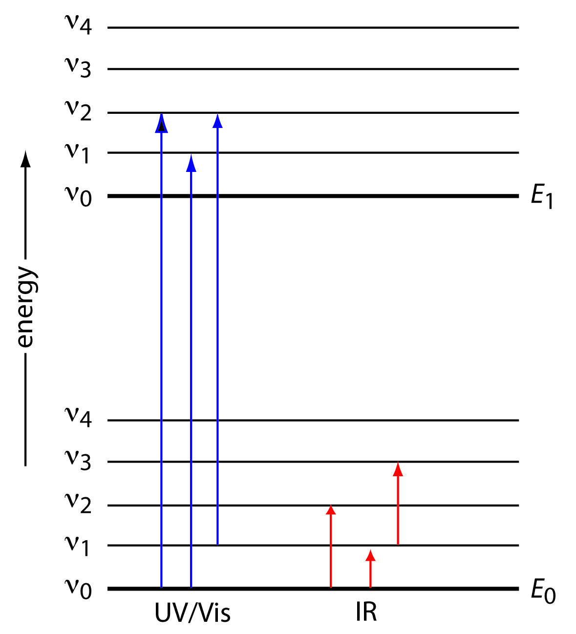
Figure 10.15 Diagram showing two electronic energy levels (E₀ and E₁), each with five vibrational energy levels (ν₀–ν₄). Absorption of ultraviolet and visible radiation leads to a change in the analyte’s electronic energy levels and, possibly, a change in vibrational energy as well. A change in vibrational energy without a change in electronic energy levels occurs with the absorption of infrared radiation.

Infrared Spectra for Molecules and Polyatomic Ions

The energy of infrared radiation produces a change in a molecule’s or a polyatomic ion’s vibrational energy, but is not sufficient to effect a change in its electronic energy. As shown in Figure 10.15, vibrational energy levels are quantized; that is, a molecule may have only certain, discrete vibrational energies. The energy for an allowed vibrational mode, E_ν, is

\[E_{\nu} = v + \dfrac{1}{2}h\nu_0\]

where ν is the vibrational quantum number, which has values of 0, 1, 2, …, and ν₀ is the bond’s fundamental vibrational frequency. The value of ν₀, which is determined by the bond’s strength and by the mass at each end of the bond, is a characteristic property of a bond. For example, a carbon-carbon single bond (C–C) absorbs infrared radiation at a lower energy than a carbon-carbon double bond (C=C) because a single bond is weaker than a double bond.

At room temperature most molecules are in their ground vibrational state (ν = 0). A transition from the ground vibrational state to the first vibrational excited state (ν = 1) requires absorption of a photon with an energy of hν₀. Transitions in which ∆ν is ±1 give rise to the fundamental absorption lines. Weaker absorption lines, called overtones, result from transitions in which ∆ν is ±2 or ±3. The number of possible normal vibrational modes for a linear molecule is 3N – 5, and for a non-linear molecule is 3N – 6, where N is the number of atoms in the molecule. Not surprisingly, infrared spectra often show a considerable number of absorption bands. Even a relatively simple molecule, such as ethanol (C₂H₆O), for example, has 3 × 9 – 6, or 21 possible normal modes of vibration, although not all of these vibrational modes give rise to an absorption. The IR spectrum for ethanol is shown in Figure 10.16.

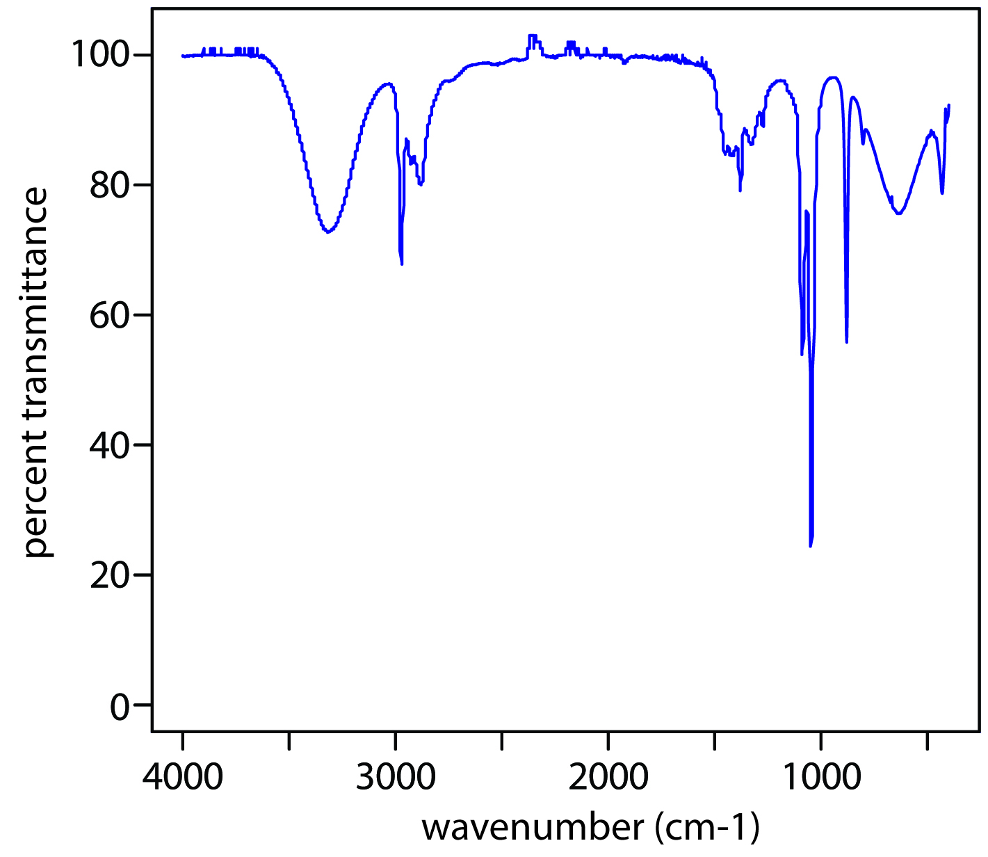
Figure 10.16 Infrared spectrum of ethanol.

Example: Methane

Why does a non-linear molecule have 3N – 6 vibrational modes? Consider a molecule of methane, CH₄. Each of the five atoms in methane can move in one of three directions (x, y, and z) for a total of 5 × 3 = 15 different ways in which the molecule can move. A molecule can move in three ways: it can move from one place to another, what we call translational motion; it can rotate around an axis; and its bonds can stretch and bend, what we call vibrational motion.

Because the entire molecule can move in the x, y, and z directions, three of methane’s 15 different motions are translational. In addition, the molecule can rotate about its x, y, and z axes, accounting for three additional forms of motion. This leaves 15 – 3 – 3 = 9 vibrational modes.

A linear molecule, such as CO₂, has 3N – 5 vibrational modes because it can rotate around only two axes.

UV/Vis Spectra for Molecules and Ions

The valence electrons in organic molecules and polyatomic ions, such as CO₃^2–, occupy quantized sigma bonding, σ, pi bonding, π, and non-bonding, n, molecular orbitals (MOs). Unoccupied sigma antibonding, σ*, and pi antibonding, π*, molecular orbitals are slightly higher in energy. Because the difference in energy between the highest-energy occupied MOs and the lowest-energy unoccupied MOs corresponds to ultraviolet and visible radiation, absorption of a photon is possible.

Four types of transitions between quantized energy levels account for most molecular UV/Vis spectra. Table 10.5 lists the approximate wavelength ranges for these transitions, as well as a partial list of bonds, functional groups, or molecules responsible for these transitions. Of these transitions, the most important are n→π^∗ and π→π^∗ because they involve important functional groups that are characteristic of many analytes and because the wavelengths are easily accessible. The bonds and functional groups that give rise to the absorption of ultraviolet and visible radiation are called chromophores.

Table 10.5 Electronic Transitions Involving n, σ, and π Molecular Orbitals

Transition	Wavelength Range	Examples
σ → σ^∗	<200 nm	C–C, C–H
n → σ^∗	160–260 nm	H2O, CH3OH, CH3Cl
π → π^∗	200–500 nm	C=C, C=O, C=N, C≡C
n → π^∗	250–600 nm	C=O, C=N, N=N, N=O

Many transition metal ions, such as Cu²⁺ and Co²⁺, form colorful solutions because the metal ion absorbs visible light. The transitions giving rise to this absorption are valence electrons in the metal ionfs d−orbitals. For a free metal ion, the five d−orbitals are of equal energy. In the presence of a complexing ligand or solvent molecule, however, the d−orbitals split into two or more groups that differ in energy and with a magnitude that can be quantified by crystal field theory. For example, in an octahedral complex of Cu(H₂O)₆²⁺ the six water molecules perturb the d−orbitals into two groups, as shown in Figure 10.17. The resulting d−d transitions for transition metal ions are relatively weak.

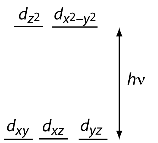
Figure 10.17 Splitting of the d-orbitals in an octahedral field.

A more important source of UV/Vis absorption for inorganic metal–ligand complexes is charge transfer, in which absorption of a photon produces an excited state in which there is transfer of an electron from the metal, M, to the ligand, L.

\[M—L + hν → (M^+—L^–)^*\]

Charge-transfer absorption is important because it produces very large absorbances. One important example of a charge-transfer complex is that of o-phenanthroline with Fe²⁺, the UV/Vis spectrum for which is shown in Figure 10.18. Charge-transfer absorption in which an electron moves from the ligand to the metal also is possible.

Note

Why is a larger absorbance desirable? An analytical method is more sensitive if a smaller concentration of analyte gives a larger signal.

Comparing the IR spectrum in Figure 10.16 to the UV/Vis spectrum in Figure 10.18 shows us that UV/Vis absorption bands are often significantly broader than those for IR absorption. We can use Figure 10.15 to explain why this is true. When a species absorbs UV/Vis radiation, the transition between electronic energy levels may also include a transition between vibrational energy levels. The result is a number of closely spaced absorption bands that merge together to form a single broad absorption band.

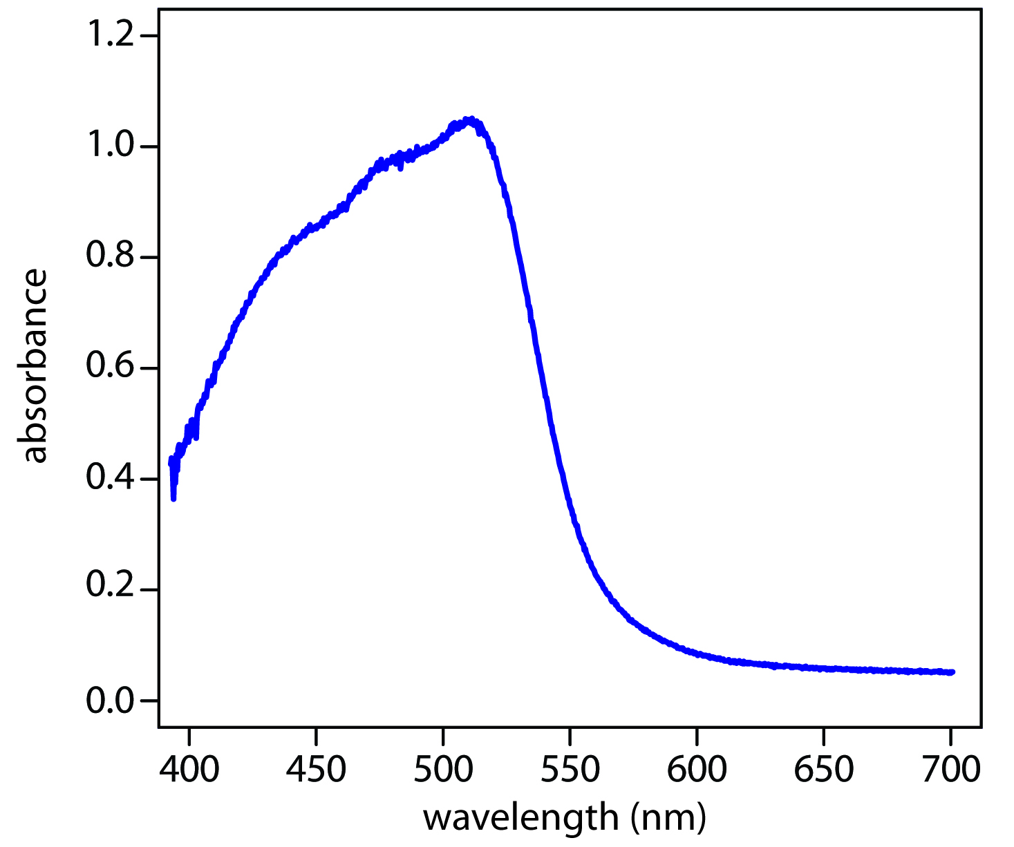
Figure 10.18 UV/Vis spectrum for the metal–ligand complex Fe(phen)₃²⁺, where phen is the ligand o-phenanthroline.

UV/Vis Spectra for Atoms

The energy of ultraviolet and visible electromagnetic radiation is sufficient to cause a change in an atom’s valence electron configuration. Sodium, for example, has a single valence electron in its 3s atomic orbital. As shown in Figure 10.19, unoccupied, higher energy atomic orbitals also exist.

Figure 10.19 Valence shell energy level diagram for sodium. The wavelengths (in wavenumbers) corresponding to several transitions are shown.

The valence shell energy level diagram in Figure 10.19 might strike you as odd because it shows that the 3p orbitals are split into two groups of slightly different energy. The reasons for this splitting are unimportant in the context of our treatment of atomic absorption. For further information about the reasons for this splitting, consult the chapter’s additional resources.

Absorption of a photon is accompanied by the excitation of an electron from a lower-energy atomic orbital to an orbital of higher energy. Not all possible transitions between atomic orbitals are allowed. For sodium the only allowed transitions are those in which there is a change of ±1 in the orbital quantum number (l); thus transitions from s → p orbitals are allowed, and transitions from s → d orbitals are forbidden.

The atomic absorption spectrum for Na is shown in Figure 10.20, and is typical of that found for most atoms. The most obvious feature of this spectrum is that it consists of a small number of discrete absorption lines corresponding to transitions between the ground state (the 3s atomic orbital) and the 3p and 4p atomic orbitals. Absorption from excited states, such as the 3p → 4s and the 3p → 3d transitions included in Figure 10.19, are too weak to detect. Because an excited state's lifetime is short—typically an excited state atom takes 10⁻⁷ to 10⁻⁸ s to return to a lower energy state—an atom in the exited state is likely to return to the ground state before it has an opportunity to absorb a photon.

Figure 10.20 Atomic absorption spectrum for sodium. Note that the scale on the x-axis includes a break.

Another feature of the atomic absorption spectrum in Figure 10.20 is the narrow width of the absorption lines, which is a consequence of the fixed difference in energy between the ground and excited states. Natural line widths for atomic absorption, which are governed by the uncertainty principle, are approximately 10^–5 nm. Other contributions to broadening increase this line width to approximately 10^–3 nm.

10.2.2 Transmittance and Absorbance

As light passes through a sample, its power decreases as some of it is absorbed. This attenuation of radiation is described quantitatively by two separate, but related terms: transmittance and absorbance. As shown in Figure 10.21a, transmittance is the ratio of the source radiation’s power exiting the sample, P_T, to that incident on the sample, P₀.

\[T = \dfrac{P_\ce{T}}{P_0} \tag{10.1}\]

Multiplying the transmittance by 100 gives the percent transmittance, %T, which varies between 100% (no absorption) and 0% (complete absorption). All methods of detecting photons—including the human eye and modern photoelectric transducers—measure the transmittance of electromagnetic radiation.

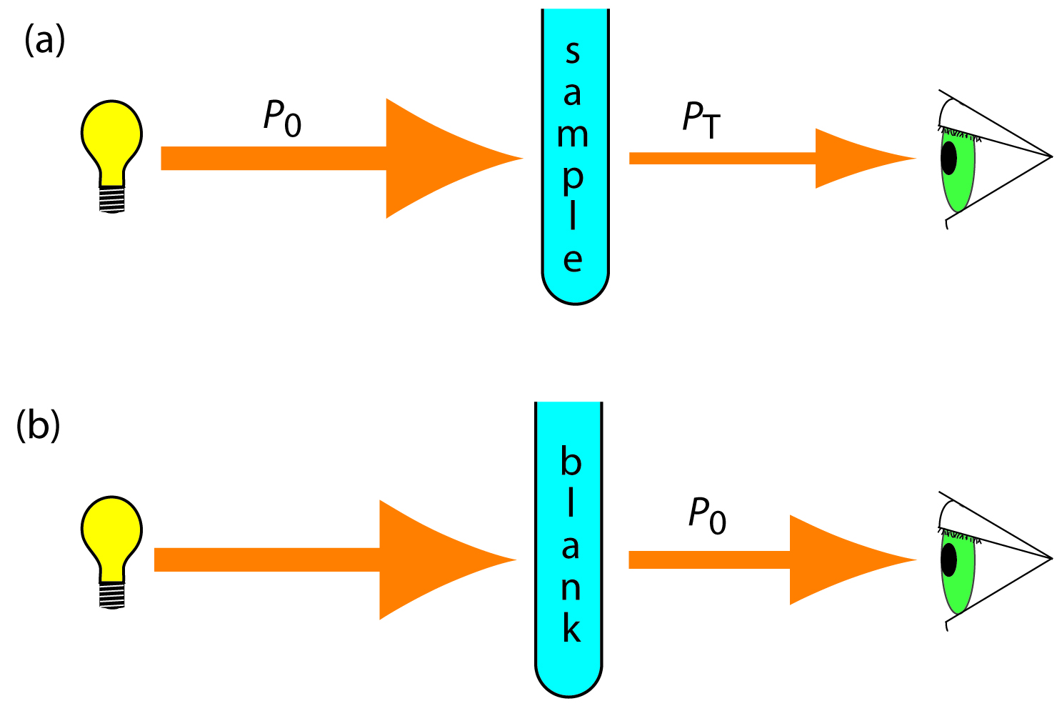
Figure 10.21 (a) Schematic diagram showing the attenuation of radiation passing through a sample; P₀ is the radiant power from the source and P_T is the radiant power transmitted by the sample. (b) Schematic diagram showing how we redefine P₀ as the radiant power transmitted by the blank. Redefining P₀ in this way corrects the transmittance in (a) for the loss of radiation due to scattering, reflection, or absorption by the sample’s container and absorption by the sample’s matrix.

Equation 10.1 does not distinguish between different mechanisms that prevent a photon emitted by the source from reaching the detector. In addition to absorption by the analyte, several additional phenomena contribute to the attenuation of radiation, including reflection and absorption by the sample’s container, absorption by other components in the sample’s matrix, and the scattering of radiation. To compensate for this loss of the radiation’s power, we use a method blank. As shown in Figure 10.21b, we redefine P₀ as the power exiting the method blank.

An alternative method for expressing the attenuation of electromagnetic radiation is absorbance, \(A\), which we define as

\[A = −\log T= −\log \dfrac{P_\ce{T}}{ P_0} \tag{10.2}\]

Absorbance is the more common unit for expressing the attenuation of radiation because it is a linear function of the analyte’s concentration. We will show that this is true in Section 10.2.3.

Example 10.3

A sample has a percent transmittance of 50%. What is its absorbance?

SOLUTION

A percent transmittance of 50.0% is the same as a transmittance of 0.500 Substituting into equation 10.2 gives

\[A = −\log T = −\log (0.500) = 0.301\]

Exercise 10.3

What is the %T for a sample if its absorbance is 1.27?

Click here to review your answer to this exercise.

Equation 10.1 has an important consequence for atomic absorption. As we saw in Figure 10.20, atomic absorption lines are very narrow. Even with a high quality monochromator, the effective bandwidth for a continuum source is 100–1000× greater than the width of an atomic absorption line. As a result, little of the radiation from a continuum source is absorbed (P₀ ≈ P_T), and the measured absorbance is effectively zero. For this reason, atomic absorption requires a line source instead of a continuum source.

10.2.3 Absorbance and Concentration: Beer’s Law

When monochromatic electromagnetic radiation passes through an infinitesimally thin layer of sample of thickness dx, it experiences a decrease in its power of dP (Figure 10.22). The fractional decrease in power is proportional to the sample’s thickness and the analyte’s concentration, C; thus]

\[− \dfrac{dP}{P} = αCdx \tag{10.3}\]

where \(P\) is the power incident on the thin layer of sample, and \(\alpha\) is a proportionality constant. Integrating the left side of equation 10.3 over the entire sample

\[−\int ^{P_\ce{T}}_{P_o} \dfrac{dP}{P} =\alpha C \int_o^b dx\]

\[\ln \dfrac{P_0}{P_\ce{T}} = αbC\]

converting from \(\ln\) to \(\log_{10}\), and substituting in equation 10.2, gives

\[A = abC \tag{10.4}\]

where a is the analyte’s absorptivity with units of cm^–1 conc^–1. If we express the concentration using molarity, then we replace a with the molar absorptivity, ε, which has units of cm^–1 M^–1.

\[A = \epsilon bC \tag{10.5}\]

The absorptivity and molar absorptivity are proportional to the probability that the analyte absorbs a photon of a given energy. As a result, values for both a and ε depend on the wavelength of the absorbed photon.

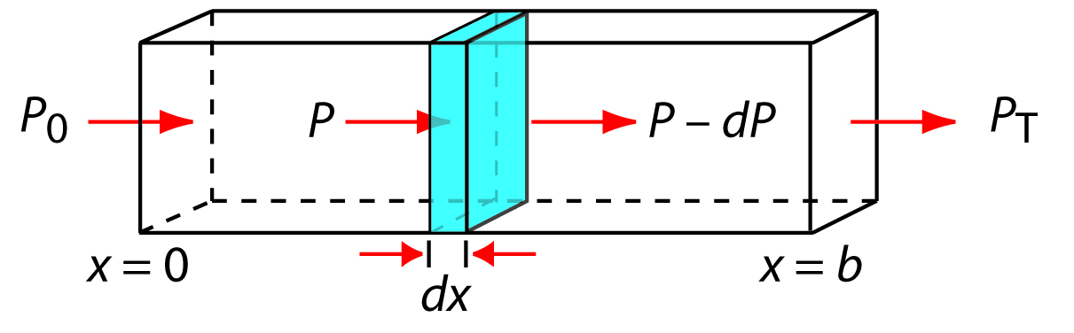
Figure 10.22 Factors used in deriving the Beer-Lambert law.

Example 10.4

A 5.00 × 10^–4 M solution of an analyte is placed in a sample cell with a pathlength of 1.00 cm. When measured at a wavelength of 490 nm, the solution’s absorbance is 0.338. What is the analyte’s molar absorptivity at this wavelength?

SOLUTION

Solving equation 10.5 for ε and making appropriate substitutions gives

\[ε = \dfrac{A}{bC} = \mathrm{\dfrac{0.338}{(1.00\: cm)(5.00×10^{−4}\: M)} = 676\: cm^{−1}\: M^{−1}}\]

Exercise 10.4

A solution of the analyte from Example 10.4 has an absorbance of 0.228 in a 1.00-cm sample cell. What is the analyte’s concentration?

Click here to review your answer to this exercise.

Equation 10.4 and equation 10.5, which establish the linear relationship between absorbance and concentration, are known as the Beer-Lambert law, or more commonly, as Beer’s law. Calibration curves based on Beer’s law are common in quantitative analyses.

10.2.4 Beer’s Law and Multicomponent Samples

We can extend Beer’s law to a sample containing several absorbing components. If there are no interactions between the components, the individual absorbances, A_i, are additive. For a two-component mixture of analyte’s X and Y, the total absorbance, A_tot, is

\[A_\ce{tot} = A_\ce{X} + A_\ce{Y} = \epsilon_\ce{X}bC_\ce{X} + \epsilon_\ce{Y}bC_\ce{Y}\]

Generalizing, the absorbance for a mixture of n components, A_mix, is

\[A_\ce{mix} = \sum_{i=0}^n A_i= \sum_{i=1}^n ε_ibC_i \tag{10.6}\]

10.2.5 Limitations to Beer’s Law

Beer’s law suggests that a calibration curve is a straight line with a y-intercept of zero and a slope of ab or εb. In many cases a calibration curve deviates from this ideal behavior (Figure 10.23). Deviations from linearity are divided into three categories: fundamental, chemical, and instrumental.

Figure 10.23 Calibration curves showing positive and negative deviations from the ideal Beer’s law calibration curve, which is a straight line.

Fundamental Limitations to Beer’s Law

Beer’s law is a limiting law that is valid only for low concentrations of analyte. There are two contributions to this fundamental limitation to Beer’s law.

1. At higher concentrations the individual particles of analyte no longer behave independently of each other. The resulting interaction between particles of analyte may change the analyte’s absorptivity.
2. A second contribution is that the analyte’s absorptivity depends on the sample’s refractive index. Because the refractive index varies with the analyte’s concentration, the values of a and ε may change. For sufficiently low concentrations of analyte, the refractive index is essentially constant and the calibration curve is linear.

Chemical Limitations to Beer’s Law

A chemical deviation from Beer’s law may occur if the analyte is involved in an equilibrium reaction. Consider, as an example, an analysis for the weak acid, HA. To construct a Beer’s law calibration curve we prepare a series of standards—each containing a known total concentration of HA—and measure each standard’s absorbance at the same wavelength. Because HA is a weak acid, it is in equilibrium with its conjugate weak base, A^–.

\[\ce{HA}_{(aq)} + \ce{H_2O}_{(l)} \rightleftharpoons \ce{H_3O^+}_{(aq)} + \ce{A^-}_{(aq)}\]

If both HA and A^– absorb at the chosen wavelength, then Beer’s law is

\[A = \epsilon_\ce{HA}bC_\ce{HA} + \epsilon_\ce{A}bC_\ce{A} \tag{10.7}\]

where C_HA and C_A are the equilibrium concentrations of HA and A^–. Because the weak acid’s total concentration, C_total, is

\[C_\ce{total} = C_\ce{HA} + C_\ce{A}\]

the concentrations of HA and A^– can be written as

\[C_\ce{HA} = \alpha_\ce{HA}C_\ce{total} \tag{10.8}\]

\[C_\ce{A} = (1−\alpha_\ce{HA})C_\ce{total} \tag{10.9}\]

where \(\alpha_{HA}\) is the fraction of weak acid present as HA. Substituting equation 10.8 and equation 10.9 into equation 10.7 and rearranging, gives

\[A = (\epsilon_\ce{HA} \alpha_\ce{HA} + \epsilon_\ce{A} − \epsilon_\ce{A} \alpha_\ce{HA} )bC_\ce{total} \tag{10.10}\]

To obtain a linear Beer’s law calibration curve, one of two conditions must be met. If α_HA and α_A have the same value at the chosen wavelength, then equation 10.10 simplifies to

\[A = \epsilon_\ce{A}bC_\ce{total}\]

Alternatively, if α_HA has the same value for all standards, then each term within the parentheses of equation 10.10 is constant—which we replace with k—and a linear calibration curve is obtained at any wavelength.

\[A = kbC_\ce{total}\]

Because HA is a weak acid, the value of α_HA varies with pH. To hold α_HA constant we buffer each standard to the same pH. Depending on the relative values of α_HAand α_A, the calibration curve has a positive or a negative deviation from Beer’s law if we do not buffer the standards to the same pH.

Note

For a monoprotic weak acid, the equation for \(\alpha_{HA}\) is

\[\alpha_\ce{HA} = \dfrac{[\ce{H_3O^+}]}{[\ce{H_3O^+}] + K_\ce{a}}\]

Problem 10.6 in the end of chapter problems asks you to explore this chemical limitation to Beer’s law.

Instrumental Limitations to Beer’s Law

There are two principal instrumental limitations to Beer’s law. The first limitation is that Beer’s law assumes that the radiation reaching the sample is of a single wavelength—that is, that the radiation is purely monochromatic. As shown in Figure 10.10, however, even the best wavelength selector passes radiation with a small, but finite effective bandwidth. Polychromatic radiation always gives a negative deviation from Beer’s law, but the effect is smaller if the value of ε is essentially constant over the wavelength range passed by the wavelength selector. For this reason, as shown in Figure 10.24, it is better to make absorbance measurements at the top of a broad absorption peak. In addition, the deviation from Beer’s law is less serious if the source’s effective bandwidth is less than one-tenth of the natural bandwidth of the absorbing species.⁵ When measurements must be made on a slope, linearity is improved by using a narrower effective bandwidth.

Note

Another reason for measuring absorbance at the top of an absorbance peak is that it provides for a more sensitive analysis. Note that the green calibration curve in Figure 10.24 has a steeper slope—a greater sensitivity—than the red calibration curve. Problem 10.7 in the end of chapter problems ask you to explore the effect of polychromatic radiation on the linearity of Beer’s law.

Figure 10.24 Effect of the choice of wavelength on the linearity of a Beer’s law calibration curve.

Stray radiation is the second contribution to instrumental deviations from Beer’s law. Stray radiation arises from imperfections in the wavelength selector that allow light to enter the instrument and reach the detector without passing through the sample. Stray radiation adds an additional contribution, P_stray, to the radiant power reaching the detector; thus

\[A = −\log \left( \dfrac{P_\ce{T} + P_\ce{stray}}{P_0+ P_\ce{stray}} \right)\]

For a small concentration of analyte, P_stray is significantly smaller than P₀ and P_T, and the absorbance is unaffected by the stray radiation. At a higher concentration of analyte, however, less light passes through the sample and P_T and P_stray may be similar in magnitude. This results is an absorbance that is smaller than expected, and a negative deviation from Beer’s law.

Note

Problem 10.8 in the end of chapter problems ask you to explore the effect of stray radiation on the linearity of Beer’s law.

Contributors

David Harvey (DePauw University)