1.12: Introduction to the Thermodynamics of Phase Transitions

Phase Diagrams

The different phases of substances are characterized by different ranges of thermodynamic variables in which these phases are the stable phases. These ranges can be represented on a diagram in which two or more of the thermodynamic state variables are plotted against each other and these different regions are indicated, together with boundary lines separating them. Such a diagram is called a phase diagram.

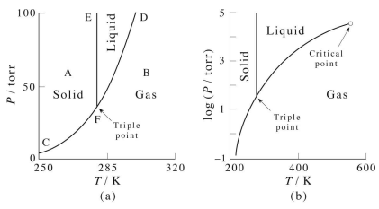
An example of a phase diagram for a normal substance, here benzene, is shown in the figure below. The diagram shows definite ranges of pressure \(P\) and temperature \(T\) for which the solid, liquid, and gas phases are stable. The line separating the solid and liquid phases is called the melting curve, that separating the liquid and gas phases is called the boiling curve, and that separating the gas and solid phases is called the sublimation curve. Along these lines, the two phases on either side coexist. Hence, these lines are also often referred to as coexistence curves. These three lines meet in a point called the triple point, at which all three phases coexist. In the right panel, we can expand the temperature axis by plotting \(\text{ln} \: P\) against \(T\), and when we do this, we see that the liquid-gas coexistence curve ends in a point, known as the critical point. In the region of the phase diagram to the right of this point, the system exists in a phase known as a supercritical fluid. In our study of the van der Waals equation, we showed that the critical point is the point at which we just begin to see the onset of cooperative effects that lead to a phase transition from gas to liquid.

Figure 13.1: Phase diagram of benzene showing \(P\) vs. \(T\) (left) and \(\text{ln} \: P\) vs. \(T\) (right).

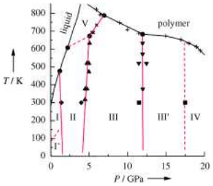
A simple phase diagram such as that shown in Figure 13.1 belies a rich complexity of behavior, particularly, in the solid region of the phase diagram, where a variety of solid structures can exist. These are the polymorphs first discussed in lecture 12 on free energies. Each of these solid phases will correspond to a different region in the phase diagram in which it is the most stable of the different solid phases. These different phases will appear in the phase diagram when the pressure axis is expanded. The figure below, for example, shows the solid part of the phase diagram for benzene, showing a wide variety of polymorphs. Each of these different solid phases has its own unique crystal structure, unit cell, and space group.

In normal systems, the slope of the solid-liquid coexistence curve is slightly positive for the reason that the solid phase has a greater density than the liquid phase near the coexistence temperature. If this is the case, then at higher pressures, it takes a higher temperature to get the system to undergo a transition from solid to liquid, since the solid phase will be preferred under conditions of extreme compression.

Figure 13.2: Solid phase diagram of benzene.

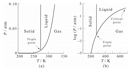
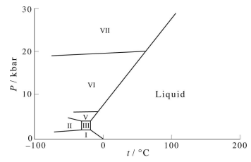
However, there are a few liquids whose solid phase is less dense than the liquid phase in the coexistence region. One of these is water, which is the reason that ice floats in water. In fact, water has its maximum density at around \(4^\text{o}C\) rather than at \(0^\text{o}C\), its freezing point at standard pressure. The water phase diagram is shown in the figure below: Here we see the slight slope to the left of the solid-liquid coexistence line. As with benzene, the solid region of the phase diagram of water also exhibits a rich variety of different structures, the ice polymorphs, not shown in the phase diagram above. Again, however, if the pressure axis is expanded, these show up. The figure below shows just a few of the known ice polymorphs (more were discussed in class):

Figure 13.3: Phase diagram of water.

Gibbs Free Energy and Phase Transitions

The Gibbs free energy is a particularly important function in the study of phases and phase transitions. The behavior of \(G(N, P,T)\), particularly as a function of \(P\) and \(T\), can signify a phase transition and can tell us some of the thermodynamic properties of different phases.

Figure 13.4: Some of the ice polymorphs.

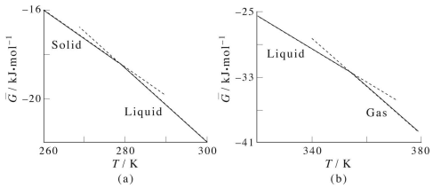
Consider, first, the behavior of \(G\) vs. \(T\) between the solid and liquid phases of benzene: We immediately notice several things. First, although the free energy is continuous across the phase transition, its first derivative, \(\partial G/\partial T\) is not: The slope of \(G(T)\) in the solid region is different from the slope in the liquid region. When the first derivative of the free energy with respect to one of its dependent thermodynamic variables is discontinuous across a phase transition, this is an example of what is called a first order phase transition. The solid-liquid-gas phase transition of most substances is first order. When the free energy exhibits continuous first derivatives but discontinuous second derivatives, the phase transition is called second order. Examples of this type of phase transition are the order-disorder transition in paramagnetic materials.

Figure 13.5: Behavior of the Gibbs free energy across the solid-liquid phase (left) and liquid-gas (right) transitions for benzene.

Now, recall that

\[S = -\dfrac{\partial G}{\partial T} \label{13.1}\]

Consider the slopes in the solid and liquid parts of the graph:

\[\dfrac{\partial G^\text{(solid)}}{\partial T} = -S^\text{(solid)}, \: \: \: \: \: \: \: \dfrac{\partial G^\text{(liquid)}}{\partial T} = -S^\text{(liquid)} \label{13.2}\]

However, since

\[\dfrac{\partial G^\text{(liquid)}}{\partial T} < \dfrac{\partial G^\text{(solid)}}{\partial T} \label{13.3}\]

(note that the slopes are all negative, and the slope of the liquid line is more negative than that of the solid line), it follows that \(-S^\text{(liquid)} < -S^\text{(solid)}\) or \(S^\text{(liquid)} > S^\text{(solid)}\). This is what we might expect considering that the liquid phase is higher in entropy than the solid phase. The same argument can be made with regards to the gaseous phase.

Similarly, if we consider the dependence of \(G\) on pressure, we obtain a curve like that shown in the figure below:

Figure 13.6: Dependence of the Gibbs free energy as a function of pressure for benzene (left) and water (right). For benzene, the temperature is above the triple point, whereas for water, it is set below triple point.

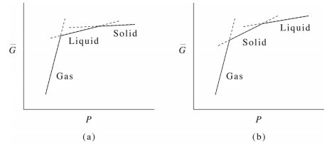
As noted previously, here again, we see that the first derivative of \(\bar{G} (P)\) is discontinuous, signifying a first-order phase transition. Recalling that the average molar volume is

\[\bar{V} = \dfrac{\partial \bar{G}}{\partial P} \label{13.4}\]

From the graph, we see that the slopes obey

\[\bar{V}^\text{(gas)} \gg \bar{V}^\text{(liquid)} > \bar{V}^\text{(solid)} \label{13.5}\]

as one might expect for a normal substance like benzene at a temperature above its triple point. Because the temperature is above the triple point, the free energy follows a continuous path (even though it is not everywhere differentiable) from gas to liquid to solid.

On the other hand, for water, we see something a bit different, namely, that

\[\bar{V}^\text{(gas)} \gg \bar{V}^\text{(solid)} > \bar{V}^\text{(liquid)} \label{13.6}\]

at a temperature below the triple point. This, again, indicates, the unusual property of water that its solid phase is less dense than its liquid phase in the coexistence region.

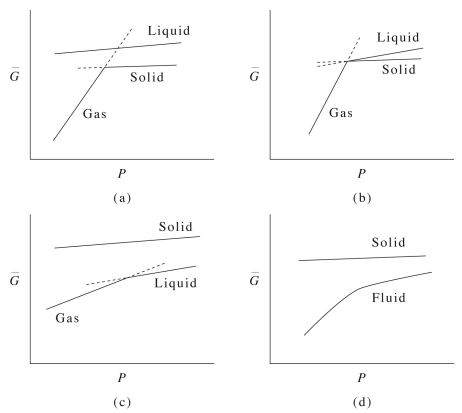
Interestingly, if we look at how the plot of \(G(P)\) changes with \(T\), we obtain a plot like that shown below: Below the triple point, it is easy to see from the benzene phase diagram that the system proceeds directly from solid to gas. There is a liquid curve on this plot that is completely disconnected from the gas-solid curve, suggesting that, below the triple point, the liquid state can exist metastably if at all. AT the triple point, the solid can transition into the liquid or gas phases depending on the value of the free energy. Near the critical temperature, we see the liquid-gas transition line, while the solid line is disconnected. Above the critical temperature, the system exists as a supercritical fluid, which is shown on the lower line, and this line now shows derivative discontinuity.

Figure 13.7: Behavior of the Gibbs free energy as a function of \(P\) across different phases at different temperatures for benzene. (a): Temperature is less than the triple point; (b): Temperature is equal to the triple point; (c): Temperature is just below the critical temperature; (d): Temperature is greater than the critical temperature.

\(n\)-Dependence of the Gibbs Free Energy

Recall that we can express \(G(N, P, T)\) equivalently as \(G(n, P, T)\), where \(n\) is the number of moles. According to Euler’s theorem,

\[G(n, P, T) = n \dfrac{\partial G}{\partial n} = n \mu (P, T) \label{13.7}\]

Therefore,

\[\dfrac{\partial G}{\partial n} = \mu (P, T) \label{13.8}\]

Now consider the liquid phase of a substance in equilibrium with its vapor. Let there be \(n_l\) moles of liquid, and \(n_g\) moles of gas. If \(n\) is the total number of moles of the substance in the system, then \(n_l + n_g = n\). Suppose now that \(dn_l\) moles of liquid are transferred to the gas phase. Since \(dn = 0\), it follows that

\[\begin{array}{rcl} dn_l + dn_g & = & 0 \\ dn_l & = & -dn_g \end{array} \label{13.9}\]

The Gibbs free energy \(G\) depends on both \(n_l\) and \(n_g\), i.e., \(G = G(n_l , n_g, P, T)\). In addition, the total Gibbs free energy \(G(n_l, n_g, P, T)\) is a sum of Gibbs free energies for the liquid and gas phases:

\[G(n_l, n_g, P, T) = G_l (n_l, P, T) + G_g (n_g, P, T) \label{13.10}\]

The change \(dG\) in the Gibbs free energy in this transfer is, therefore,

\[\begin{align} dG &= \left( \dfrac{\partial G}{\partial n_l} \right)_{P, T} dn_l + \left( \dfrac{\partial G}{\partial n_g} \right)_{P, T} dn_g \\ &= \left( \dfrac{\partial G_l}{\partial n_l} \right)_{P, T} dn_l + \left( \dfrac{\partial G_g}{\partial n_g} \right)_{P, T} dn_g \\ &= \mu_l (P, T) dn_l + \mu_g (P, T) dn_g \\ &= \left[ \mu_l (P, T) - \mu_g (P, T) \right] dn_l \end{align} \label{13.11}\]

In equilibrium, \(dG = 0\), so from the above, it follows that

\[\begin{array}{rcl} \left[ \mu_l (P, T) - \mu_g (P, T) \right] dn_l & = & 0 \\ \mu_l (P, T) & = & \mu_g (P, T) \end{array} \label{13.12}\]

Hence, in equilibrium, the chemical potentials in the liquid and gas phases are equal. Recall, however, that the chemical potential is the work needed to increase the number of moles of a substance by \(1\) moles. Therefore, in equilibrium the work needed to increase the number of moles of the gas and liquid phases is the same.

Away from equilibrium, the sign of \(dG\) tells us the direction of the matter transfer. Thus, if \(dG < 0\), then matter transfer is spontaneous. Here, we need to consider two cases. First, suppose \(\mu_g > \mu_l\). Then, for \(dG\) to be negative, \(dn_l > 0\), which means that the liquid will increase by \(dn_l\) until \(dG = 0\). This is what we would expect given that the work needed to add matter to the liquid phase is less than that of the gas phase. On the other hand, suppose \(\mu_g < \mu_l\). Then, we need \(dn_l < 0\), and the liquid phase will decrease by \(dn_l\) moles until \(dG = 0\). Again, less work is needed to add matter to the gas phase in this case, hence, the direction of matter transfer is as expected.

Enthalpies and Phase Changes

Recall that the Gibbs free energy has two contributions since \(G = H - TS\). The behavior of the enthalpy \(H\) is also interesting when phase changes occur because of the discontinuous change in the isobaric heat capacity \(C_P (T)\) across a phase boundary.

The constant-pressure heat capacity \(C_P\) is given by

\[C_P = \left( \dfrac{\partial H}{\partial T} \right)_P \label{13.13}\]

For an ideal gas, \(C_P\) is independent of temperature, however, for non-ideal systems, \(C_P\) does depend on \(T\) :

\[C_P (T) = \left( \dfrac{\partial H}{\partial T} \right)_P \label{13.14}\]

If we wish to consider the reaction enthalpy at a temperature other than that of the standard state, where enthalpies are tabulated, we can use Equation \(\ref{13.14}\) to obtain the enthalpy at the desired temperature. Integrating both sides of Equation \(\ref{13.14}\) from a temperature \(T_1\) to \(T_2\), we obtain

\[ \int_{T_1}^{T_2} C_P (T) \: dT = \int_{T_1}^{T_2} \left( \dfrac{\partial H}{\partial T} \right)_P dT\]

\[ \int_{T_1}^{T_2} C_P (T) \: dT = H(T_2) - H(T_1) \label{13.15}\]

The use of Equation \(\ref{13.15}\), of course, assumes that the \(H(T)\) is everywhere smooth and differentiable, so that it can be integrated.

Figure 13.8: Plot of molar enthalpy \(\bar{H} (T) - \bar{H} (0)\) for benzene. Discontinuities in the plot occur at points of phase transitions from solid to liquid \(T_\text{melt}\) and from liquid to gas \(T_\text{vap}\).

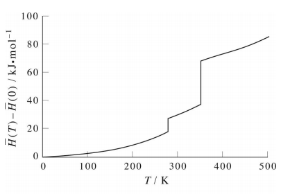
However, if we plot the molar enthalpy difference \(\bar{H} (T) - \bar{H} (0)\) for a real substance such as benzene, we find a curve like that shown in figure above. There are two temperatures at which \(H(T)\) exhibits a discontinuity. These two temperatures are the melting temperature \(T_\text{melt}\) of the solid and the vaporization temperature \(T_\text{vap}\) of the liquid. According to our discussion of phase changes, the heat needed to effect these two phase changes are \(\Delta_\text{fus} H\) and \(\Delta_\text{vap} H\), respectively. At these temperatures, \(C_P = \partial H/\partial T\) diverges, and we cannot smoothly integrate through these divergences. In fact, divergence of the heat capacity is one of the signatures of a phase transition. As long as \(T < T_\text{melt}\), we can smoothly integrate \(C_P (T)\) to obtain a value for \(H(T)\):

\[H(T) - H(0) = \int_0^T C_P (T') \: dT' \label{13.16}\]

However, if we are interested in a temperature \(T > T_\text{melt}\), then we must treat the discontinuity as a special point. Fortunately, we already know the enthalpy change at this point, i.e., \(\Delta_\text{fus} H\), and we can simply add it in. Thus, for \(T > T_\text{melt}\), we would calculate \(H(T)\) as follows:

\[H(T) - H(0) = \int_0^{T_\text{melt}} C_P (T') \: dT' + \Delta_\text{fus} H + \int_{T_\text{melt}}^T C_P (T') \: dT' \label{13.17}\]

The same holds for \(T > T_\text{vap}\). When we reach the discontinuity at \(T_\text{vap}\), we simply add in the enthalpy of vaporization \(\Delta_\text{vap} H\):

\[H(T) - H(0) = \int_0^{T_\text{melt}} C_P (T') \: dT' + \Delta_\text{fus} H + \int_{T_\text{melt}}^{T_\text{vap}} C_P (T') \: dT' + \Delta_\text{vap} H + \int_{T_\text{vap}}^T C_P (T') \: dT' \label{13.18}\]

Example 13.1

Consider the reaction

\[CO (g) + H_2 O (g) \longrightarrow H_2 (g) + CO_2 (g) /n\nonumber\]

For this reaction, the heat capacity has the following temperature dependence

\[C_P (T) = a + bT + cT^2 \label{13.19} /n\nonumber\]

where \(a\), \(b\), and \(c\) are constants. Calculate the reaction enthalpy at \(800 \: \text{K}\) for this reaction given the following data: For \(CO\): \(a = 26.86\), \(b = 6.99 \times 10^{-3}\), \(c = 8.20 \times 10^{-7}\), for \(H_2 O\): \(a = 30.98\), \(b = 9.62 \times 10^{-3}\), \(c = 11.84 \times 10^{-7}\), for \(CO_2\): \(a = 25.98\), \(b = 43.51 \times 10^{-3}\), \(c = -184.32 \times 10^{-7}\), for \(H_2\): \(a = 26.08\), \(b = -0.84 \times 10^{-3}\), \(c = 20.13 \times 10^{-7}\). The units of \(a\), \(b\), and \(c\) are \(\text{J} \cdot \text{mol}^{-1} \cdot \text{K}^{-1}\), \(\text{J} \cdot \text{mol}^{-1} \cdot \text{K}^{-2}\), and \(\text{J} \cdot \text{mol}^{-1} \cdot \text{K}^{-3}\), respectively. Standard-state formation enthalpies for \(CO\), \(H_2 O\), \(CO_2\), and \(H_2\) are \(-110.52 \: \text{kJ/mol}\), \(-241.82 \: \text{kJ/mol}\), \(-393.51 \: \text{kJ/mol}\), and \(0 \: \text{kJ/mol}\), respectively.

Solution

Since this is already a gas-phase reaction, we do not need to worry about melting or vaporization, so we can smoothly integrate \(C_P (T)\) from the standard state, where \(T = 298 \: \text{K}\) to the desired \(800 \: \text{K}\). Let us first obtain the formation enthalpies at \(800 \: \text{K}\). Since our reference state is \(298 \: \text{K}\), the integral we need is

\[\Delta_\text{f} H^\text{(800)} = \Delta_\text{f} H^\text{o} + \int_{T_0}^{T_f} C_P (T) \: dT\]

where \(T_0 = 298 \: \text{K}\) and \(T_f = 800 \: \text{K}\). The integral is

\[\int_{T_0}^{T_f} C_P (T) \: dT = a(T_f - T_0) + \dfrac{1}{2} b(T_f^2 - T_0^2) + \dfrac{1}{3} c (T_f^3 - T_0^3)\]

Plugging in the data, we obtain

\[\begin{array}{rcl} \Delta_\text{f} H^\text{(800)} (CO) & = & -94.981 \: \text{kJ/mol} \\ \Delta_\text{f} H^\text{(800)} (CO_2) & = & -370.883 \: \text{kJ/mol} \\ \Delta_\text{f} H^\text{(800)} (H_2 O) & = & -223.731 \: \text{kJ/mol} \\ \Delta_\text{f} H^\text{(800)} (H_2) & = & 14.668 \: \text{kJ/mol} \end{array} \label{13.20}\]

Therefore, the overall reaction enthalpy is

\[\begin{array}{rcl} \Delta_\text{f} H^\text{(800)} & = & \Delta_\text{f} H^\text{(800)} (H_2) + \Delta_\text{f} H^\text{(800)} (CO_2) - \Delta_\text{f} H^\text{(800)} (H_2 O) - \Delta_\text{f} H^\text{(800)} (CO) \\ & = & 14.668 - 370.883 + 94.981 + 223.731 = -37.503 \: \text{kJ/mol} \end{array}\]