1.11: Carnot engines, thermodynamic entropy, and the second and third laws

Carnot Engines and the Thermodynamic Definition of Entropy

We have been using two definitions of the entropy almost interchangeable. One is a purely thermodynamic definition involving the heat absorbed by a system in a reversible process at temperature \(T\) :

\[\Delta S = \int_A^B \frac{dQ_\text{rev}}{T} \label{12.1}\]

while the other is purely statistical. Given two states \(A\) and \(B\) with numbers of microstates \(\Omega_A\) and \(\Omega_B\), the change in entropy is determined from Boltzmann’s relation:

\[\Delta S = S_B - S_A = k_B \: \text{ln} \: \Omega_B - k_B \: \text{ln} \: \Omega_A = k_B \: \text{ln} \: \left( \frac{\Omega_B}{\Omega_A} \right) \label{12.2}\]

Two questions then naturally arise. Where does the thermodynamic definition actually come from, and are these two definitions really equivalent? In order to explore this, we will study a particular thermodynamic cycle called an engine.

In general, the processes that engines undergo are highly irreversible. As an idealization, we will consider the operation of a particular kind of engine, called a Carnot engine, that operates reversibly between its initial, intermediate and final states. By analyzing such a device, it should be possible to place an upper bound on the efficiency of any engine operating between a high temperature reservoir at \(T_h\) and a low temperature reservoir at \(T_l\).

Consider the thermodynamic path shown below:

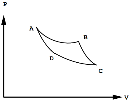
Figure 12.1: The Carnot cycle.

This closed thermodynamic path or cycle is called the Carnot cycle. In the \(ABC\) portion of the cycle, the system expands, so it does work. In the \(CDA\) portion of the path, the system is compressed, so work is done on it. The net work, which is the sum of contributions from paths \(ABC\) and path \(CDA\), is the net work done by the system, so it must be negative:

\[W_\text{net} = -\int_{\text{path} \: ABC} P \: dV - \int_{\text{path} \: CDA} P \: dV \label{12.3}\]

Note that the net work performed by the engine is just the area of enclosed by the by four paths in the \(P - V\) plane. Since, for a closed path, the change in energy is \(0\), the net work done by the gas must be equal the negative of the heat absorbed by the system:

\[W = -W_\text{net} = -q \label{12.4}\]

Now suppose that the system is an ideal gas. We have already developed expressions for the work done by/on the the system for various parts of this thermodynamic cycle:

• Path \(AB\): Isothermal expansion at temperature \(T_h\):

\[W_{AB} = -q_{AB} = -nRT_h \: \text{ln} \: \left( \frac{V_B}{V_A} \right) \label{12.5}\]

• Path \(BC\): Adiabatic expansion:

\[\begin{array}{rcl} q_{BC} & = & 0 \\ W_{BC} & = & nc_V (T_l - T_h) \end{array} \label{12.6}\]

• Path \(CD\): Isotherm compression at temperature \(T_l\):

\[W_{CD} = -q_{CD} = -nRT_l \: \text{ln} \: \left( \frac{V_D}{V_C} \right) \label{12.7}\]

• Path \(DA\): Adiabatic compression:

\[\begin{array}{rcl} q_{DA} & = & 0 \\ W_{DA} & = & nc_V (T_h - T_l) \end{array} \label{12.8}\]

The net work done on the system is

\[\begin{align} W_\text{net} &= W_{AB} + W_{BC} + W_{CD} + W_{DA} \\ &= -nRT_h \: \text{ln} \: \left( \frac{V_B}{V_A} \right) + nRT_l \: \text{ln} \: \left( \frac{V_C}{V_D} \right) \end{align} \label{12.9}\]

Recall, however, that in an adiabatic expansion, the temperatures \(T_1\) and \(T_2\) are related to the volumes \(V_1\) and \(V_2\) by

\[\frac{T_2}{T_1} = \left( \frac{V_1}{V_2} \right)^{\gamma - 1} \label{12.10}\]

which can be applied to the paths \(BC\) and \(DA\), the adiabatic expansion and compression parts of the cycle. Thus, for the path \(BC\),

\[\frac{T_h}{T_l} = \left( \frac{V_C}{V_B} \right)^{\gamma - 1} \label{12.11}\]

and for the path \(DA\),

\[\frac{T_h}{T_l} = \left( \frac{V_D}{V_A} \right)^{\gamma - 1} \label{12.12}\]

from which it follows that

\[\frac{V_C}{V_B} = \frac{V_D}{V_A} \label{12.13}\]

or

\[\frac{V_B}{V_A} = \frac{V_C}{V_D} \label{12.14}\]

and the net work done on the system is

\[W_\text{net} = -nR (T_h - T_l) \: \text{ln} \: \left( \frac{V_B}{V_A} \right) \label{12.15}\]

Note also that, since a complete cycle has been made, \(\Delta E = 0\) for the cycle. Thus, from the first law of thermodynamics,

\[-W_\text{net} = q_{AB} + q_{CD} \label{12.16}\]

which is the net heat absorbed by the system. Since heat is only absorbed/discharged during the isothermal parts of the cycle, only \(q_{AB}\) and \(q_{CD}\) are nonzero.

In the first part of the next lecture, the derivation will continue, beginning with a determination of the maximum efficiency of a Carnot engine.

The efficiency of a device is defined to be the net work it can produce per unit of heat taken in:

\[\epsilon = -\frac{W_\text{net}}{q_{AB}} \label{12.17}\]

Thus, if all of the heat taken in is converted to useful work with no discharge of waste heat, then the device is 100% efficient. We will now show that such a case is not possible.

For the Carnot cycle, in which a system containing an ideal gas undergoes reversible transformations around the cycle, we have

\[\begin{align} W_\text{net} &= -nR(T_h - T_l) \: \text{ln} \: \left( \frac{V_B}{V_A} \right) \\ q_{AB} &= nRT_h \: \text{ln} \: \left( \frac{V_B}{V_A} \right) \end{align} \label{12.18}\]

And the negative ratio of these, which gives the efficiency, is

\[\epsilon = \frac{nR(T_h - T_l) \: \text{ln} \: (V_B/V_A)}{nRT_h \: \text{ln} \: (V_B/V_A)} = \frac{T_h -T_l}{T_h} = 1 - \frac{T_l}{T_h} \label{12.19}\]

Thus, for an engine operating reversibly between a high temperature \(T_h\) and a low temperature \(T_l\), the maximum efficiency of such a machine is \(1 - (T_l/T_h)\). In order to achieve, 100% efficiency, therefore, it would be necessary to make \(T_l =0\) or \(T_h = \infty\), neither of which is possible. However, the larger the temperature difference, the greater will be the efficiency of the device. The difficulty with large temperature differences, in general, is that they are difficult to make, and it is also difficult to find materials that can withstand both extremely high AND extremely low temperatures.

Although this result was derived for a system containing an ideal gas, it turns out to be true for all Carnot engines operating reversibly between \(T_h\) and \(T_l\). To prove this result, the technique of proof by contradiction will be used.

Assume that there are two engines operating reversibly between \(T_h\) and \(T_l\) with different efficiencies, \(\epsilon_1\) and \(\epsilon_2\) such that \(\epsilon_1 > \epsilon_2\). The machines are adjusted so that work output of both is equal, \(-W_1 = -W_2\). We let the more efficient machine, \(1\), be operated as a normal Carnot engine, withdrawing heat at \(T_h\), discarding waste heat at \(T_l\) and producing an output \(-W_1\) of useful work. The less efficient engine is run in reverse, as a “heat pump,” withdrawing heat at the low temperature \(T_l\), consuming useful work from an outside source, and delivering a quantity of heat to the high temperature \(T_h\). This is how a refrigerator operates. In this case, the work output of machine \(1\) is used to operate machine \(2\). The figure below illustrates this:

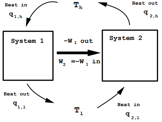
Figure 12.2: Illustrating the Carnot engine.

Since \(-W_1 =W_2\), the net work output of the two machines combined is \(W_\text{tot} = 0\). Also, since each machine completes a thermodynamic cycle, the total energy change of the two machines combined is also \(0\) (\(\Delta E_\text{tot} = 0\)). Since \(\epsilon_1 > \epsilon_2\),

\[\begin{align} \frac{-W_1}{q_{1,h}} &> \frac{W_2}{-q_{2,h}} \\ -W_1 &= W_2 \\ \Rightarrow \frac{1}{q_{1,h}} &> \frac{1}{q_{2,h}} \\ q_{1,h} &< q_{2,h} \end{align} \label{12.20}\]

But from the first law of thermodynamics, since \(\Delta E_\text{tot} = 0\) and \(W_\text{tot} = 0\), the total heat absorbed by the system \(q_\text{tot} = 0\). The total heat absorbed is

\[q_{1,h} - q_{1,l} + q_{2,l} - q_{2,h} = 0 \label{12.21}\]

Thus,

\[q_{1,h} - q_{2,h} = q_{1,l} - q_{2,l} \label{12.22}\]

The left side is the net heat absorbed at \(T_h\) and the right side is the net heat discharged at \(T_l\). Since \(q_{1,h} < q_{2,h}\), the left side is negative, and so the right side must be negative as well, and

\[q_{1,l} < q_{2,l} \label{12.23}\]

Since \(q_{2,h} > q_{1,h}\) there is a net amount of heat delivered to the high temperature reservoir, and a net amount of heat extracted from the low temperature reservoir. In other words, the combined machine is capable of extracting an amount of heat from a cold source and delivering it to a hot source with NO expenditure of work!!!!!

While there is no logical contradiction here, the result would seem to imply that it must be possible for heat to flow from cold to hot without input of work, which has never been observed. Rather, only the opposite has been observed, heat flowing naturally from hot to cold. Thus, we are lead to conclude that all Carnot engines must have the same efficiency.

Derivation of the Thermodynamic Definition of Entropy

We saw in the analysis above that, for a Carnot cycle:

\[-W_\text{net} = q_h + q_l \label{12.24}\]

Thus, the efficiency can be expressed as

\[\epsilon = \frac{-W_\text{net}}{q_h} = \frac{q_h + q_l}{q_h} = \frac{T_h - T_l}{T_h} \label{12.25}\]

which implies that

\[1 + \frac{q_l}{q_h} = 1 - \frac{T_l}{T_h} \label{12.26}\]

or

\[\begin{align} \frac{q_l}{q_h} &= -\frac{T_l}{T_h} \\ \frac{q_l}{T_l} &= -\frac{q_h}{T_h} \\ \frac{q_l}{T_l} + \frac{q_h}{T_h} &= 0 \end{align} \label{12.27}\]

Recall that a state function is a thermodynamic quantity, whose change between initial and final states is independent of the path between the states. By extension, it follows that a state function is one whose change around any closed thermodynamic path is \(0\). Thus, since \(q/T\) is zero for the Carnot cycle, it would seem that \(q/T\) is a state function. In fact, this turns out to be true. To see this, note that any Carnot cycle can be composed of an infinite number of Carnot cycles for which the isothermal parts of the cycle are of infinitesimally small length (see Figure 8.6 in the text). The quantity of heat absorbed along each of these isotherms is \(\delta q_i\) for the \(i^\text{th}\) cycle. Since \(\delta q_{i,h}/T_{i,h} + \delta q_{i.l}/T_{i.l} = 0\) for the \(i^\text{th}\) cycle, summing over all cycles gives

\[\sum_i \left[ \frac{\delta q_{i,h}}{T_{i,h}} + \frac{\delta q_{i.l}}{T_{i.l}} \right] = 0 \label{12.28}\]

which approaches the integral expression as the number of cycles becomes infinitely large:

\[\oint \frac{dq_\text{rev}}{T} = 0 \label{12.29}\]

where \(\oint\) indicates that the integral is taken over a closed thermodynamic cycle. This, then, leads to the Clausius definition entropy, as the state function, \(\Delta S = S_f - S_i\), given by

\[\Delta S = \int_i^f \frac{dq_\text{rev}}{T} \label{12.30}\]

Clearly, then \(\Delta S = 0\) over any closed path. In the next section, we will show that this definition of \(\Delta S\) is consistent with the statistical (Boltzmann) definition for an ideal gas.

Isothermal Processes in an Ideal Gas

In an isothermal process, the temperature is held constant so that

\[\Delta S = \int_i^f \frac{dq_\text{rev}}{T} = \frac{1}{T} \int_i^f dq_\text{rev} \label{12.31}\]

The differential \(dq_\text{rev}\) can be integrated as a perfect differential \(q_\text{rev}\), which is the heat absorbed by the system in the reversible process that takes the system from state \(i\) to state \(f\):

\[\Delta S = \frac{q_\text{rev}}{T} \label{12.32}\]

Isothermal expansion/compression of an ideal gas

In the last chapter, we derived the expression for the isothermal expansion/compression of an ideal gas from a volume \(V_1\) to a volume \(V_2\):

\[q_\text{rev} = nRT \: \text{ln} \: \left( \frac{V_2}{V_1} \right) \label{12.33}\]

From this, it follows that the entropy change in the expansion/compression is

\[\Delta S = nR \: \text{ln} \: \left( \frac{V_2}{V_1} \right) \label{12.34}\]

To see that the same expression results from the Boltzmann definition of entropy, recall that the number of microscopic states is

\[\Omega (N, V, T) = cV^N (k_B T)^{3N/2} \label{12.35}\]

At constant temperature, the number of microscopic states available to the system in the volume \(V_1\) and in the volume \(V_2\) are, respectively,

\[\begin{array}{rcl} \Omega_1 & = & cV_1^N (k_B T)^{3N/2} \\ \Omega_2 & = & cV_2^N (k_B T)^{3N/2} \end{array} \label{12.36}\]

Thus,

\[\begin{align} \Delta S &= k_B \: \text{ln} \: \left( \frac{\Omega_2}{\Omega_1} \right) \\ &= k_B \: \text{ln} \: \left( \frac{V_2}{V_1} \right)^N \\ &= N k_B \: \text{ln} \: \left( \frac{V_2}{V_1} \right) \\ &= nR \: \text{ln} \: \left( \frac{V_2}{V_1} \right) \end{align} \label{12.37}\]

which agrees with the thermodynamic definition perfectly.

Isochoric heat absorption/emission of an ideal gas

An isochoric process is one that occurs at constant volume. Consider the heat absorption/emission of an ideal gas at constant volume. A small amount of heat \(dq_\text{rev}\) absorbed a change in temperature \(dT\) related to the heat \(dq_\text{rev}\) by

\[dq_\text{rev} = nc_V dT \label{12.38}\]



Thus, the entropy change when the temperature goes from \(T_1\) to \(T_2\) is

\[\begin{align} \Delta S &= \int_{T_1}^{T_2} \frac{nc_V dT}{T} \\ &= nc_V \: \text{ln} \: \left( \frac{T_2}{T_1} \right) \end{align} \label{12.39}\]

From the Boltzmann definition, the number of microstates at temperatures \(T_1\) and \(T_2\) and volume \(V\) are, respectively,

\[\begin{array}{rcl} \Omega_1 & = & cV^N (k_B T_1)^{3N/2} \\ \Omega_2 & = & cV^N (k_B T_2)^{3N/2} \end{array} \label{12.40}\]

so that

\[\begin{align} \Delta S &= k_B \: \text{ln} \: \left( \frac{\Omega_2}{\Omega_1} \right) \\ &= k_B \: \text{ln} \: \left( \frac{T_2}{T_1} \right)^{3N/2} \\ &= \frac{3}{2} N k_B \: \text{ln} \: \left( \frac{T_2}{T_1} \right) \\ &= \frac{3}{2} nR \: \text{ln} \: \left( \frac{T_2}{T_1} \right) \end{align} \label{12.41}\]

Recalling that \(c_V\) for an ideal gas is

\[c_V = \frac{3}{2} R \label{12.42}\]

gives

\[\Delta S = n c_V \: \text{ln} \: \left( \frac{T_2}{T_1} \right) \label{12.43}\]

which, again, agrees with the thermodynamic definition.

Isobaric heat absorption/emission of an ideal gas

By analogy with the isochoric process, the entropy change in an isobaric process can be shown to be

\[\Delta S = nc_P \: \text{ln} \: \left( \frac{T_2}{T_1} \right) \label{12.44}\]

In order to derive this from the Boltzmann definition, we need to express the number of microstates of an ideal gas at constant pressure. At constant volume, we have

\[\Omega (N, V, T) = cV^N (k_B T)^{3N/2} \label{12.45}\]

However, from the ideal gas law:

\[V = \frac{N k_B T}{P} \label{12.46}\]

Thus, the number of microstates becomes

\[\Omega (N, P, T) = CP^{-N} (k_B T)^{5N/2} \label{12.47}\]

where \(C\) is another constant. Thus, at constant pressure \(P\) and temperatures \(T_1\) and \(T_2\), the respective numbers of microstates are

\[\begin{array}{rcl} \Omega_1 & = & CP^{-N} (k_B T_1)^{5N/2} \\ \Omega_2 & = & CP^{-N} (k_B T_2)^{5N/2} \end{array} \label{12.48}\]

Thus, the entropy change is

\[\begin{align} \Delta S &= k_B \: \text{ln} \: \left( \frac{T_2}{T_1} \right)^{5N/2} \\ &= \frac{5}{2} N k_B \: \text{ln} \: \left( \frac{T_2}{T_1} \right) \\ &= \frac{5}{2} nR \: \text{ln} \: \left( \frac{T_2}{T_1} \right) \end{align} \label{12.49}\]

However, recognizing that \(5R/2\) is just the constant pressure heat capacity \(c_P\), we have

\[\Delta S = n c_P \: \text{ln} \: \left( \frac{T_2}{T_1} \right) \label{12.50}\]

which, again, agrees with the thermodynamic definition.

Adiabatic expansion/compression of an ideal gas

Recall that in an adiabatic expansion/compression, no heat is absorbed or emitted. Hence, \(dq_\text{rev} = 0\) and \(\Delta S = 0\). In order to derive this result from the Boltzmann definition, we note that \(P\), \(V\), and \(T\) all change in the adiabatic process, hence,

\[\begin{array}{rcl} \Omega_1 & = & cV_1^N (k_B T_1)^{3N/2} \\ \Omega_2 & = & cV_2^N (k_B T_2)^{3N/2} \end{array} \label{12.51}\]

The ratio is

\[\frac{\Omega_2}{\Omega_1} = \frac{V_2^N (k_B T_2)^{3N/2}}{V_1^N (k_B T_1)^{3N/2}} = \left[ \frac{V_2}{V_1} \frac{T_2^{3/2}}{T_1^{3/2}} \right] \label{12.52}\]

However, in an adiabatic process, we showed that the temperatures and volumes are related by

\[T_1V_1^{\gamma - 1} = T_2 V_2^{\gamma - 1} \label{12.53}\]

where \(\gamma = 5/3\) for an ideal gas. This implies that

\[\begin{align} T_1V_1^{2/3} &= T_2V_2^{2/3} \\ T_1^{3/2} V_1 &= T_2^{3/2} V_2 \\ 1 &= \frac{T_2^{3/2}}{T_1^{3/2}} \frac{V_2}{V_1} \end{align} \label{12.54}\]

which is just the ratio \(\Omega_2/\Omega_1\). Therefore, from the Boltzmann definition:

\[\Delta S = k_B \: \text{ln} \: \left( \frac{\Omega_2}{\Omega_1} \right) = k_B \: \text{ln} \: (1) = 0 \label{12.55}\]

The Second and Third Laws of Thermodynamics

We noted that entropy is a thermodynamic state function related to the number of microscopic states available to a system. Thus, any process that gives rise to an increase in the number of microscopic states in a system will also lead to an increase in the entropy. In order to quantify this, let us consider another simple thought experiment.

Consider the irreversible, isothermal expansion of an ideal gas. This can be achieved by allowing the external pressure \(P_\text{ext}\) to drop suddenly below the internal pressure \(P^\text{(int)}\). The work done on the gas in the expansion is

\[W_\text{irrev} = -\int P_\text{ext} dV \label{12.56}\]

If we compare such a process to a reversible expansion in which the gas is always in equilibrium with its surroundings, then \(P^\text{(int)} \approx P_\text{ext}\), and

\[W_\text{rev} = -\int P^\text{(int)} dV \label{12.57}\]

In the irreversible process, since \(P_\text{ext}\) drops quickly, \(P_\text{ext} < P^\text{(int)}\) and hence,

\[\begin{array}{rcl} -W_\text{irrev} & < & -W_\text{rev} \\ W_\text{irrev} & > & W_\text{rev} \end{array} \label{12.58}\]

Now let \(Q_\text{rev}\) and \(Q_\text{irrev}\) be the amounts of heat absorbed by the gas in the reversible and irreversible processes, respectively. Since energy is a state function, the first law tells us that the change in energy can be computed along the reversible or irreversible path with the same result:

\[\Delta E = Q_\text{rev} + W_\text{rev} = Q_\text{irrev} + W_\text{irrev} \label{12.59}\]

Since \(W_\text{irrev} > W_\text{rev}\), it must follow that \(Q_\text{irrev} < Q_\text{rev}\). Thus, for small changes, \(dQ_\text{irrev} < dQ_\text{rev}\). Therefore, in an isothermal process

\[\frac{dQ_\text{irrev}}{T} < \frac{dQ_\text{rev}}{T} \label{12.60}\]

Since

\[dS = \frac{dQ_\text{rev}}{T} \label{12.61}\]

it follows that

\[dS > \frac{dQ_\text{irrev}}{T} \label{12.62}\]

Generally,

\[dS \geq \frac{dQ}{T} \label{12.63}\]

or

\[\Delta S \geq \int \frac{dQ}{T} \label{12.64}\]

where equality holds only for reversible processes. This inequality is called the Clausius inequality.

Now, we apply the Clausius inequality to the entire thermodynamic universe (system \(+\) surroundings). Since the universe must be self-contained and isolated, \(dQ =0\) for the full universe, and this means that

\[\Delta S \geq 0, \: \: \: \: \: \: \: \text{(Thermodynamic Universe)} \label{12.65}\]

Again, equality holds in any reversible process. Equation 12.65 is known as the second law of thermodynamics. It is a statement, not about the system alone, but about the full thermodynamic universe. The second law states that the only direction for spontaneous changes in the entropy is an increase. Processes for which \(\Delta S < 0\) are not possible. Now since \(S = k_B \: \text{ln} \: \Omega\),

\[\Delta S = k_B \: \text{ln} \: \left( \frac{\Omega_\text{final}}{\Omega_\text{initial}} \right) \geq 0 \label{12.66}\]

We see that an irreversible process must increase the number of microscopic states available to the thermodynamic universe.

The third law of thermodynamics asks what happens to the entropy as \(T \rightarrow 0\), and this can be easily seen from the Boltzmann relation \(S = k_B \: \text{ln} \: \Omega\) and our definition of classical microstates. Since

\[\left< \sum_{i=1}^N \frac{\textbf{p}_i^2}{2m_i} \right> = \frac{3}{2} N k_B T \label{12.67}\]

and the energy is equipartitioned among all of the kinetic energy contributions, as \(T \rightarrow 0\), the only possibility is that all of the momenta (and velocities) of the particles become identically \(0\). When this happens, the particles stop moving, and their positions become “frozen” into one particular choice. Thus, in the sense of a microcanonical ensemble, there can be only one microstate available to the system, and this will be the global minimum of the potential energy \(U(\textbf{r}_1, \ldots, \textbf{r}_N)\). Thus, we see that \(\Omega \rightarrow 1\), and, therefore, \(S \rightarrow 0\), which is known as the third law of thermodynamics.

The third law of thermodynamics makes it possible to calculate entropy changes thermodynamics, as it provides us with a reference states at which we always know the absolute entropy, namely, at \(T =0\). Recall from the first law of thermodynamics that if the number of moles of a system remains fixed, then

\[\Delta E = Q_\text{rev} + W_\text{rev} = Q_\text{rev} - P \: dV \label{12.68}\]

Thus,

\[Q_\text{rev} = \Delta (E + PV) = \Delta H \label{12.69}\]

where \(H\) is the enthalpy. Thus, for an infinitesimal change, \(dQ_\text{rev} = dH\). However, the definition of the constant- pressure heat capacity is

\[C_P (T) = \left( \frac{\partial H}{\partial T} \right)_P \label{12.70}\]

This implies that we can compute entropy changes from the heat capacity as

\[\Delta S = \int_0^T \frac{dQ_\text{rev}}{T} = \int_0^T \frac{C_P (T')}{T'} dT' \label{12.71}\]

This relation will become important as we begin to study phase transitions.