3.2: The Bohr Model

Learning Objectives

• Describe the Bohr model of the hydrogen atom

Following the work of Ernest Rutherford and his colleagues in the early twentieth century, the picture of atoms consisting of tiny dense nuclei surrounded by lighter and even tinier electrons continually moving about the nucleus was well established. This picture was called the planetary model, since it pictured the atom as a miniature “solar system” with the electrons orbiting the nucleus like planets orbiting the sun. The simplest atom is hydrogen, consisting of a single proton as the nucleus about which a single electron moves. The electrostatic force attracting the electron to the proton depends only on the distance between the two particles.

In 1913, Niels Bohr attempted to resolve the atomic paradox by ignoring classical electromagnetism’s prediction that the orbiting electron in hydrogen would continuously emit light. Instead, he incorporated into the classical mechanics description of the atom Planck’s ideas of quantization and Einstein’s finding that light consists of photons whose energy is proportional to their frequency. Bohr assumed that the electron orbiting the nucleus would not normally emit any radiation (the stationary state hypothesis), but it would emit or absorb a photon if it moved to a different orbit.

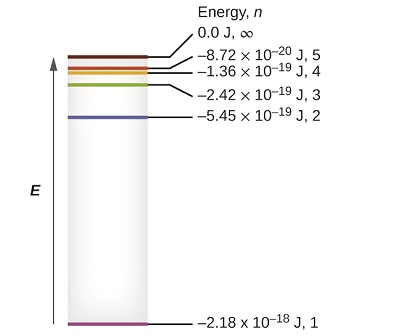
The lowest few energy levels are shown in Figure \(\PageIndex{1}\). One of the fundamental laws of physics is that matter is most stable with the lowest possible energy. Thus, the electron in a hydrogen atom usually moves in the \(n = 1\) orbit, the orbit in which it has the lowest energy. When the electron is in this lowest energy orbit, the atom is said to be in its ground electronic state (or simply ground state). If the atom receives energy from an outside source, it is possible for the electron to move to an orbit with a higher \(n\) value and the atom is now in an excited electronic state (or simply an excited state) with a higher energy. When an electron transitions from an excited state (higher energy orbit) to a less excited state, or ground state, the difference in energy is emitted as a photon. Similarly, if a photon is absorbed by an atom, the energy of the photon moves an electron from a lower energy orbit up to a more excited one.

Figure \(\PageIndex{1}\): Quantum numbers and energy levels in a hydrogen atom. The more negative the calculated value, the lower the energy.

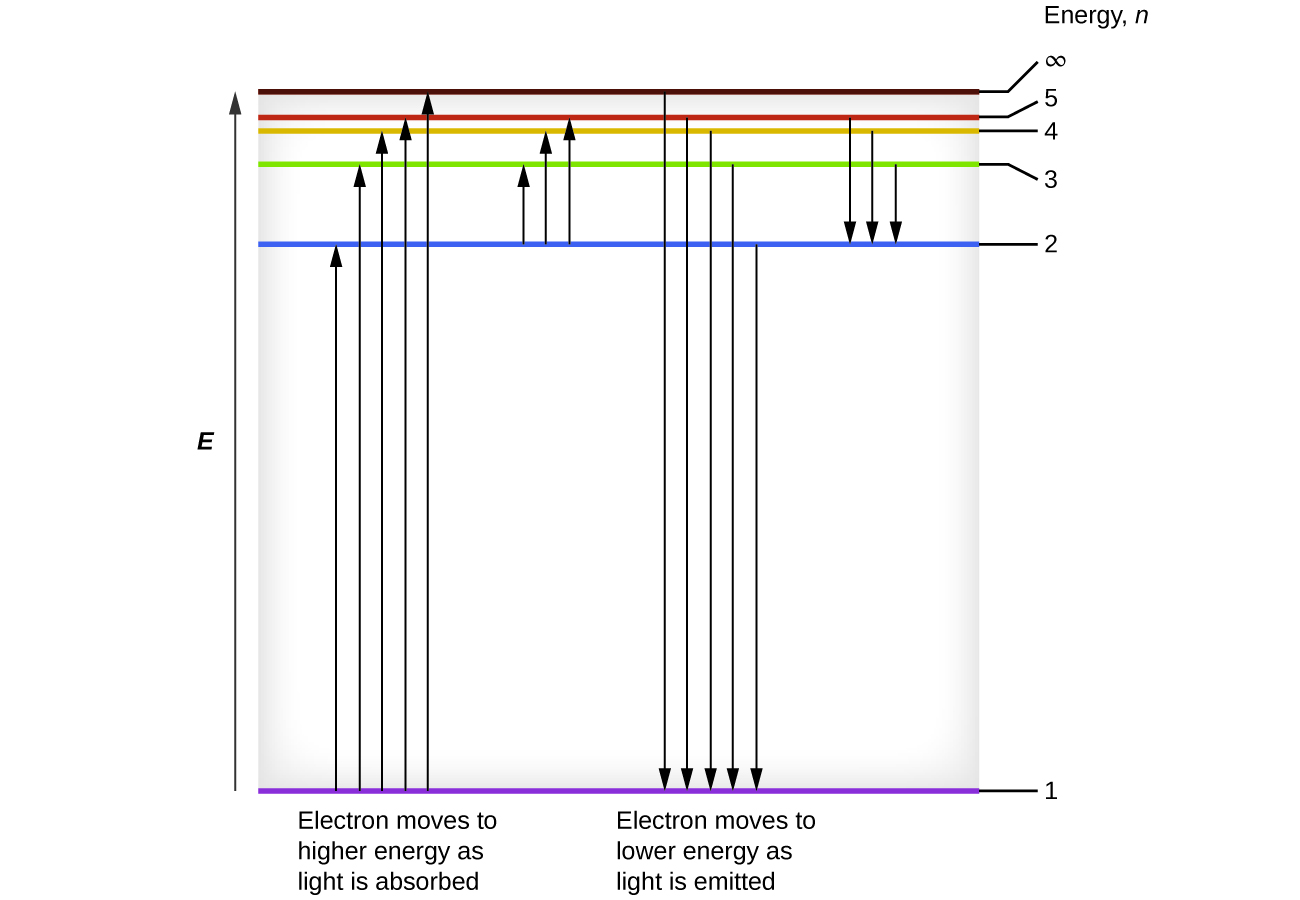
We can relate the energy of electrons in atoms to what we learned previously about energy. The law of conservation of energy says that we can neither create nor destroy energy. Thus, if a certain amount of external energy is required to excite an electron from one energy level to another, that same amount of energy will be liberated when the electron returns to its initial state (Figure \(\PageIndex{2}\)). In effect, an atom can “store” energy by using it to promote an electron to a state with a higher energy and release it when the electron returns to a lower state. The energy can be released as one quantum of energy, as the electron returns to its ground state (say, from \(n = 5\) to \(n = 1\)), or it can be released as two or more smaller quanta as the electron falls to an intermediate state, then to the ground state (say, from \(n = 5\) to \(n = 4\), emitting one quantum, then to \(n = 1\), emitting a second quantum).

Figure \(\PageIndex{2}\): The horizontal lines show the relative energy of orbits in the Bohr model of the hydrogen atom, and the vertical arrows depict the energy of photons absorbed (left) or emitted (right) as electrons move between these orbits.

Bohr’s model of the hydrogen atom provides insight into the behavior of matter at the microscopic level. It introduces several important features of all models used to describe the distribution of electrons in an atom. These features include the following:

• The energies of electrons (energy levels) in an atom are quantized, described by quantum numbers: integer numbers having only specific allowed value and used to characterize the arrangement of electrons in an atom.
• An electron’s energy increases with increasing distance from the nucleus.
• The discrete energies (lines) in the spectra of the elements result from quantized electronic energies.

Of these features, the most important is the postulate of quantized energy levels for an electron in an atom. As a consequence, the model laid the foundation for the quantum mechanical model of the atom. Later in this chapter, we will examine how these specific energy levels relate to the periods (rows) of the Periodic Table and structure of larger atoms.

Summary

The Bohr model of the hydrogen atom helps to determine why atoms produce line spectra instead of continuous spectrums. It also helps to lay the foundation for how electrons are organized in an atom into discrete levels.

Glossary

Bohr’s model of the hydrogen atom

structural model in which an electron moves around the nucleus only in circular orbits, each with a specific allowed radius; the orbiting electron does not normally emit electromagnetic radiation, but does so when changing from one orbit to another.

excited state

state having an energy greater than the ground-state energy

ground state

state in which the electrons in an atom, ion, or molecule have the lowest energy possible

quantum number

integer number having only specific allowed values and used to characterize the arrangement of electrons in an atom

Contributors and Attributions

• Paul Flowers (University of North Carolina - Pembroke), Klaus Theopold (University of Delaware) and Richard Langley (Stephen F. Austin State University) with contributing authors. Textbook content produced by OpenStax College is licensed under a Creative Commons Attribution License 4.0 license. Download for free at http://cnx.org/contents/85abf193-2bd...a7ac8df6@9.110).