
4.13: Reading- Calculating Opportunity Cost
- Page ID
- 249246
\( \newcommand{\vecs}[1]{\overset { \scriptstyle \rightharpoonup} {\mathbf{#1}} } \)
\( \newcommand{\vecd}[1]{\overset{-\!-\!\rightharpoonup}{\vphantom{a}\smash {#1}}} \)
\( \newcommand{\id}{\mathrm{id}}\) \( \newcommand{\Span}{\mathrm{span}}\)
( \newcommand{\kernel}{\mathrm{null}\,}\) \( \newcommand{\range}{\mathrm{range}\,}\)
\( \newcommand{\RealPart}{\mathrm{Re}}\) \( \newcommand{\ImaginaryPart}{\mathrm{Im}}\)
\( \newcommand{\Argument}{\mathrm{Arg}}\) \( \newcommand{\norm}[1]{\| #1 \|}\)
\( \newcommand{\inner}[2]{\langle #1, #2 \rangle}\)
\( \newcommand{\Span}{\mathrm{span}}\)
\( \newcommand{\id}{\mathrm{id}}\)
\( \newcommand{\Span}{\mathrm{span}}\)
\( \newcommand{\kernel}{\mathrm{null}\,}\)
\( \newcommand{\range}{\mathrm{range}\,}\)
\( \newcommand{\RealPart}{\mathrm{Re}}\)
\( \newcommand{\ImaginaryPart}{\mathrm{Im}}\)
\( \newcommand{\Argument}{\mathrm{Arg}}\)
\( \newcommand{\norm}[1]{\| #1 \|}\)
\( \newcommand{\inner}[2]{\langle #1, #2 \rangle}\)
\( \newcommand{\Span}{\mathrm{span}}\) \( \newcommand{\AA}{\unicode[.8,0]{x212B}}\)
\( \newcommand{\vectorA}[1]{\vec{#1}} % arrow\)
\( \newcommand{\vectorAt}[1]{\vec{\text{#1}}} % arrow\)
\( \newcommand{\vectorB}[1]{\overset { \scriptstyle \rightharpoonup} {\mathbf{#1}} } \)
\( \newcommand{\vectorC}[1]{\textbf{#1}} \)
\( \newcommand{\vectorD}[1]{\overrightarrow{#1}} \)
\( \newcommand{\vectorDt}[1]{\overrightarrow{\text{#1}}} \)
\( \newcommand{\vectE}[1]{\overset{-\!-\!\rightharpoonup}{\vphantom{a}\smash{\mathbf {#1}}}} \)
\( \newcommand{\vecs}[1]{\overset { \scriptstyle \rightharpoonup} {\mathbf{#1}} } \)
\( \newcommand{\vecd}[1]{\overset{-\!-\!\rightharpoonup}{\vphantom{a}\smash {#1}}} \)
\(\newcommand{\avec}{\mathbf a}\) \(\newcommand{\bvec}{\mathbf b}\) \(\newcommand{\cvec}{\mathbf c}\) \(\newcommand{\dvec}{\mathbf d}\) \(\newcommand{\dtil}{\widetilde{\mathbf d}}\) \(\newcommand{\evec}{\mathbf e}\) \(\newcommand{\fvec}{\mathbf f}\) \(\newcommand{\nvec}{\mathbf n}\) \(\newcommand{\pvec}{\mathbf p}\) \(\newcommand{\qvec}{\mathbf q}\) \(\newcommand{\svec}{\mathbf s}\) \(\newcommand{\tvec}{\mathbf t}\) \(\newcommand{\uvec}{\mathbf u}\) \(\newcommand{\vvec}{\mathbf v}\) \(\newcommand{\wvec}{\mathbf w}\) \(\newcommand{\xvec}{\mathbf x}\) \(\newcommand{\yvec}{\mathbf y}\) \(\newcommand{\zvec}{\mathbf z}\) \(\newcommand{\rvec}{\mathbf r}\) \(\newcommand{\mvec}{\mathbf m}\) \(\newcommand{\zerovec}{\mathbf 0}\) \(\newcommand{\onevec}{\mathbf 1}\) \(\newcommand{\real}{\mathbb R}\) \(\newcommand{\twovec}[2]{\left[\begin{array}{r}#1 \\ #2 \end{array}\right]}\) \(\newcommand{\ctwovec}[2]{\left[\begin{array}{c}#1 \\ #2 \end{array}\right]}\) \(\newcommand{\threevec}[3]{\left[\begin{array}{r}#1 \\ #2 \\ #3 \end{array}\right]}\) \(\newcommand{\cthreevec}[3]{\left[\begin{array}{c}#1 \\ #2 \\ #3 \end{array}\right]}\) \(\newcommand{\fourvec}[4]{\left[\begin{array}{r}#1 \\ #2 \\ #3 \\ #4 \end{array}\right]}\) \(\newcommand{\cfourvec}[4]{\left[\begin{array}{c}#1 \\ #2 \\ #3 \\ #4 \end{array}\right]}\) \(\newcommand{\fivevec}[5]{\left[\begin{array}{r}#1 \\ #2 \\ #3 \\ #4 \\ #5 \\ \end{array}\right]}\) \(\newcommand{\cfivevec}[5]{\left[\begin{array}{c}#1 \\ #2 \\ #3 \\ #4 \\ #5 \\ \end{array}\right]}\) \(\newcommand{\mattwo}[4]{\left[\begin{array}{rr}#1 \amp #2 \\ #3 \amp #4 \\ \end{array}\right]}\) \(\newcommand{\laspan}[1]{\text{Span}\{#1\}}\) \(\newcommand{\bcal}{\cal B}\) \(\newcommand{\ccal}{\cal C}\) \(\newcommand{\scal}{\cal S}\) \(\newcommand{\wcal}{\cal W}\) \(\newcommand{\ecal}{\cal E}\) \(\newcommand{\coords}[2]{\left\{#1\right\}_{#2}}\) \(\newcommand{\gray}[1]{\color{gray}{#1}}\) \(\newcommand{\lgray}[1]{\color{lightgray}{#1}}\) \(\newcommand{\rank}{\operatorname{rank}}\) \(\newcommand{\row}{\text{Row}}\) \(\newcommand{\col}{\text{Col}}\) \(\renewcommand{\row}{\text{Row}}\) \(\newcommand{\nul}{\text{Nul}}\) \(\newcommand{\var}{\text{Var}}\) \(\newcommand{\corr}{\text{corr}}\) \(\newcommand{\len}[1]{\left|#1\right|}\) \(\newcommand{\bbar}{\overline{\bvec}}\) \(\newcommand{\bhat}{\widehat{\bvec}}\) \(\newcommand{\bperp}{\bvec^\perp}\) \(\newcommand{\xhat}{\widehat{\xvec}}\) \(\newcommand{\vhat}{\widehat{\vvec}}\) \(\newcommand{\uhat}{\widehat{\uvec}}\) \(\newcommand{\what}{\widehat{\wvec}}\) \(\newcommand{\Sighat}{\widehat{\Sigma}}\) \(\newcommand{\lt}{<}\) \(\newcommand{\gt}{>}\) \(\newcommand{\amp}{&}\) \(\definecolor{fillinmathshade}{gray}{0.9}\)
It makes intuitive sense that Charlie can buy only a limited number of bus tickets and burgers with a limited budget. Also, the more burgers he buys, the fewer bus tickets he can buy. With a simple example like this, it isn’t too hard to determine what he can do with his very small budget, but when budgets and constraints are more complex, it’s important to know how to solve equations that demonstrate budget constraints and opportunity cost.
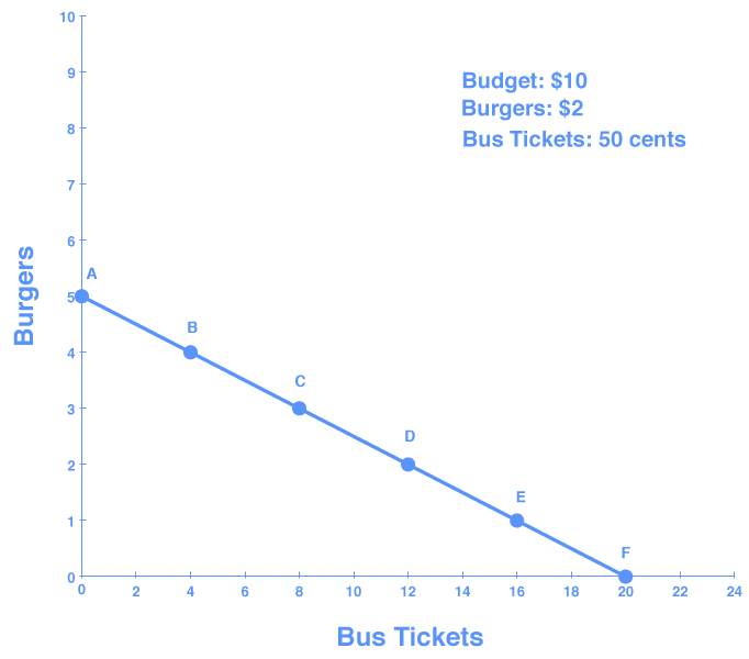
Very simply, when Charlie is spending his full budget on burgers and tickets, his budget is equal to the total amount that he spends on burgers plus the total amount that he spends on bus tickets. For example, if Charlie buys four bus tickets and four burgers with his $10 budget (point B on the graph below), the equation would be
You can see this on the graph of Charlie’s budget constraint, Figure 1, below.
If we want to answer the question “How many burgers and bus tickets can Charlie buy?” then we need to use the budget constraint equation.
Step 1. The equation for any budget constraint is the following:
where P and Q are the price and respective quantity of any number, n, of items purchased and Budget is the amount of income one has to spend.
Step 2. Apply the budget constraint equation to the scenario.
In Charlie’s case, this works out to be
For Charlie, this is
Step 3. Simplify the equation.
At this point we need to decide whether to solve for or
.
Remember, . So, in this equation
represents the number of burgers Charlie can buy depending on how many bus tickets he wants to purchase in a given week.
. So,
represents the number of bus tickets Charlie can buy depending on how many burgers he wants to purchase in a given week.
We are going solve for .
Step 4. Use the equation.
Now we have an equation that helps us calculate the number of burgers Charlie can buy depending on how many bus tickets he wants to purchase in a given week.
For example, say he wants 8 bus tickets in a given week. represents the number of bus tickets Charlie buys, so we plug in 8 for
, which gives us
This means Charlie can buy 3 burgers that week (point C on the graph, above).
Let’s try one more. Say Charlie has a week when he walks everywhere he goes so that he can splurge on burgers. He buys 0 bus tickets that week. represents the number of bus tickets Charlie buys, so we plug in 0 for
, giving us
So, if Charlie doesn’t ride the bus, he can buy 5 burgers that week (point A on the graph).
If you plug other numbers of bus tickets into the equation, you get the results shown in Table 1, below, which are the points on Charlie’s budget constraint.
| Table 1. | ||
|---|---|---|
| Point | Quantity of Burgers (at $2) | Quantity of Bus Tickets (at 50 cents) |
| A | 5 | 0 |
| B | 4 | 4 |
| C | 3 | 8 |
| D | 2 | 12 |
| E | 1 | 16 |
| F | 0 | 20 |
Step 4. Graph the results.
If we plot each point on a graph, we can see a line that shows us the number of burgers Charlie can buy depending on how many bus tickets he wants to purchase in a given week.
We can make two important observations about this graph. First, the slope of the line is negative (the line slopes downward). Remember in the last module when we discussed graphing, we noted that when when X and Y have a negative, or inverse, relationship, X and Y move in opposite directions—that is, as one rises, the other falls. This means that the only way to get more of one good is to give up some of the other.
Second, the slope is defined as the change in the number of burgers (shown on the vertical axis) Charlie can buy for every incremental change in the number of tickets (shown on the horizontal axis) he buys. If he buys one less burger, he can buy four more bus tickets. The slope of a budget constraint always shows the opportunity cost of the good that is on the horizontal axis. If Charlie has to give up lots of burgers to buy just one bus ticket, then the slope will be steeper, because the opportunity cost is greater.
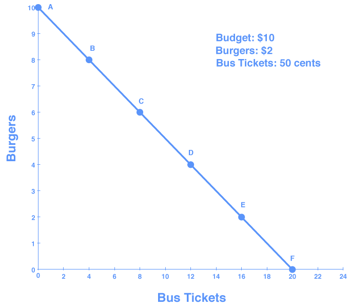
Let’s look at this in action and see it on a graph. What if we change the price of the burger to $1? We will keep the price of bus tickets at 50 cents. Now, instead of buying 4 more tickets for every burger he gives up, Charlie can only buy 2 tickets for every burger he gives up. Figure 3, below, shows Charlie’s new budget constraint (and the change in slope).
Self Check: The Cost of Choices
Answer the question(s) below to see how well you understand the topics covered in the previous section. This short quiz does not count toward your grade in the class, and you can retake it an unlimited number of times.
You’ll have more success on the Self Check if you’ve completed the two Readings in this section.
Use this quiz to check your understanding and decide whether to (1) study the previous section further or (2) move on to the next section.
- Revision and adaptation. Provided by: Lumen Learning. License: CC BY: Attribution
- Principles of Microeconomics Chapter 2.1. Authored by: OpenStax College. Provided by: Rice University. Located at: http://cnx.org/contents/6i8iXmBj@10.170:vPtYALiD@9/How-Individuals-Make-Choices-B. License: CC BY: Attribution. License Terms: Download for free at http://cnx.org/content/col11627/latest
- Ten Dollars. Authored by: Richard Grandmorin. Located at: https://www.flickr.com/photos/r_grandmorin/6831207299/. License: CC BY: Attribution