6.10: Raoult’s Law and Phase Diagrams of Ideal Solutions

The behavior of the vapor pressure of an ideal solution can be mathematically described by a simple law established by François-Marie Raoult (1830–1901). Raoult’s law states that the partial pressure of each component, \(i\), of an ideal mixture of liquids, \(P_i\), is equal to the vapor pressure of the pure component \(P_i^*\) multiplied by its mole fraction in the mixture \(x_i\):

\[ P_i=x_i P_i^*. \label{13.1.1} \]

One volatile component

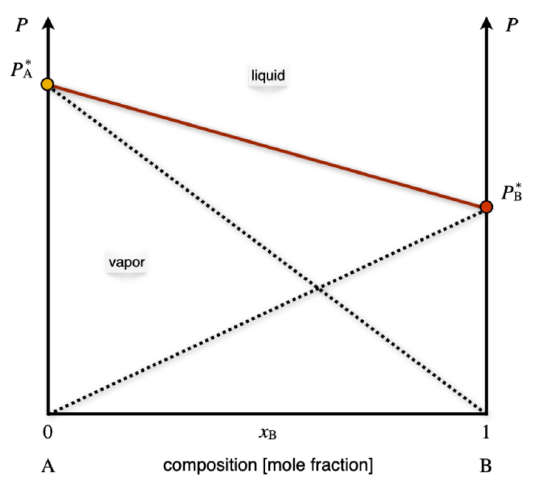
Raoult’s law applied to a system containing only one volatile component describes a line in the \(Px_{\text{B}}\) plot, as in Figure \(\PageIndex{1}\).

Figure \(\PageIndex{1}\): The Pressure–Composition Phase Diagram of an Ideal Solution Containing a Single Volatile Component at Constant Temperature.

As emerges from Figure \(\PageIndex{1}\), Raoult’s law divides the diagram into two distinct areas, each with three degrees of freedom.\(^1\) Each area contains a phase, with the vapor at the bottom (low pressure), and the liquid at the top (high pressure). Raoult’s law acts as an additional constraint for the points sitting on the line. Therefore, the number of independent variables along the line is only two. Once the temperature is fixed, and the vapor pressure is measured, the mole fraction of the volatile component in the liquid phase is determined.

Two volatile components

In an ideal solution, every volatile component follows Raoult’s law. Since the vapors in the gas phase behave ideally, the total pressure can be simply calculated using Dalton’s law as the sum of the partial pressures of the two components \(P_{\text{TOT}}=P_{\text{A}}+P_{\text{B}}\). The corresponding diagram is reported in Figure \(\PageIndex{2}\). The total vapor pressure, calculated using Dalton’s law, is reported in red. The Raoult’s behaviors of each of the two components are also reported using black dashed lines.

Figure \(\PageIndex{2}\): The Pressure–Composition Phase Diagram of an Ideal Solution Containing Two Volatile Components at Constant Temperature.

Exercise \(\PageIndex{1}\)

Calculate the mole fraction in the vapor phase of a liquid solution composed of 67% of toluene (\(\mathrm{A}\)) and 33% of benzene (\(\mathrm{B}\)), given the vapor pressures of the pure substances: \(P_{\text{A}}^*=0.03\;\text{bar}\), and \(P_{\text{B}}^*=0.10\;\text{bar}\).

Answer

The data available for the systems are summarized as follows: \[\begin{equation} \begin{aligned} x_{\text{A}}=0.67 \qquad & \qquad x_{\text{B}}=0.33 \\ P_{\text{A}}^* = 0.03\;\text{bar} \qquad & \qquad P_{\text{B}}^* = 0.10\;\text{bar} \\ & P_{\text{TOT}} = ? \\ y_{\text{A}}=? \qquad & \qquad y_{\text{B}}=? \end{aligned} \end{equation}\label{13.1.2} \] The total pressure of the vapors can be calculated combining Dalton’s and Roult’s laws: \[\begin{equation} \begin{aligned} P_{\text{TOT}} &= P_{\text{A}}+P_{\text{B}}=x_{\text{A}} P_{\text{A}}^* + x_{\text{B}} P_{\text{B}}^* \\ &= 0.67\cdot 0.03+0.33\cdot 0.10 \\ &= 0.02 + 0.03 = 0.05 \;\text{bar} \end{aligned} \end{equation}\label{13.1.3} \] We can then calculate the mole fraction of the components in the vapor phase as: \[\begin{equation} \begin{aligned} y_{\text{A}}=\dfrac{P_{\text{A}}}{P_{\text{TOT}}} & \qquad y_{\text{B}}=\dfrac{P_{\text{B}}}{P_{\text{TOT}}} \\ y_{\text{A}}=\dfrac{0.02}{0.05}=0.40 & \qquad y_{\text{B}}=\dfrac{0.03}{0.05}=0.60 \end{aligned} \end{equation}\label{13.1.4} \] Notice how the mole fraction of toluene is much higher in the liquid phase, \(x_{\text{A}}=0.67\), than in the vapor phase, \(y_{\text{A}}=0.40\).

As is clear from the results of Exercise \(\PageIndex{1}\), the concentration of the components in the gas and vapor phases are different. We can also report the mole fraction in the vapor phase as an additional line in the \(Px_{\text{B}}\) diagram of Figure \(\PageIndex{2}\). When both concentrations are reported in one diagram—as in Figure \(\PageIndex{3}\)—the line where \(x_{\text{B}}\) is obtained is called the liquidus line, while the line where the \(y_{\text{B}}\) is reported is called the Dew point line.

Figure \(\PageIndex{3}\): The Pressure–Composition Phase Diagram of an Ideal Solution Containing Two Volatile Components at Constant Temperature. Both the Liquidus and Dew Point Line are Emphasized in this Plot.

The liquidus and Dew point lines determine a new section in the phase diagram where the liquid and vapor phases coexist. Since the degrees of freedom inside the area are only 2, for a system at constant temperature, a point inside the coexistence area has fixed mole fractions for both phases. We can reduce the pressure on top of a liquid solution with concentration \(x^i_{\text{B}}\) (see Figure \(\PageIndex{3}\)) until the solution hits the liquidus line. At this pressure, the solution forms a vapor phase with mole fraction given by the corresponding point on the Dew point line, \(y^f_{\text{B}}\).

\(T_{\text{B}}\) phase diagrams and fractional distillation

We can now consider the phase diagram of a 2-component ideal solution as a function of temperature at constant pressure. The \(T_{\text{B}}\) diagram for two volatile components is reported in Figure \(\PageIndex{4}\).

Figure \(\PageIndex{4}\): The Temperature–Composition Phase Diagram of an Ideal Solution Containing Two Volatile Components at Constant Pressure.

Compared to the \(Px_{\text{B}}\) diagram of Figure \(\PageIndex{3}\), the phases are now in reversed order, with the liquid at the bottom (low temperature), and the vapor on top (high Temperature). The liquidus and Dew point lines are curved and form a lens-shaped region where liquid and vapor coexists. Once again, there is only one degree of freedom inside the lens. As such, a liquid solution of initial composition \(x_{\text{B}}^i\) can be heated until it hits the liquidus line. At this temperature the solution boils, producing a vapor with concentration \(y_{\text{B}}^f\). As is clear from Figure \(\PageIndex{4}\), the mole fraction of the \(\text{B}\) component in the gas phase is lower than the mole fraction in the liquid phase. This fact can be exploited to separate the two components of the solution. In particular, if we set up a series of consecutive evaporations and condensations, we can distill fractions of the solution with an increasingly lower concentration of the less volatile component \(\text{B}\). This is exemplified in the industrial process of fractional distillation, as schematically depicted in Figure \(\PageIndex{5}\).

Figure \(\PageIndex{5}\): The Fractional Distillation Process and Theoretical Plates Calculated on a Temperature–Composition Phase Diagram.

Each of the horizontal lines in the lens region of the \(Tx_{\text{B}}\) diagram of Figure \(\PageIndex{5}\) corresponds to a condensation/evaporation process and is called a theoretical plate. These plates are industrially realized on large columns with several floors equipped with condensation trays. The temperature decreases with the height of the column. A condensation/evaporation process will happen on each level, and a solution concentrated in the most volatile component is collected. The theoretical plates and the \(Tx_{\text{B}}\) are crucial for sizing the industrial fractional distillation columns.

---

1. Only two degrees of freedom are visible in the \(Px_{\text{B}}\) diagram. Temperature represents the third independent variable.︎