2.8.3: The 1H-NMR experiment

In an NMR experiment, a sample compound (we'll again use methyl acetate as our example) is placed inside a very strong applied magnetic field (\(B_0\)) generated by a superconducting magnet in the instrument. 

At first, the magnetic moments of (slightly more than) half of the protons in the sample are aligned with \(B_0\), and half are aligned against \(B_0\). Then, the sample is exposed to a range of radio frequencies. Out of all of the frequencies which hit the sample, only two - the resonance frequencies for H_a and H_b - are absorbed, causing those protons which are aligned with \(B_0\) to 'spin flip' so that they align themselves against \(B_0\). When the 'flipped' protons flip back down to their ground state, they emit energy, again in the form of radio-frequency radiation. The NMR instrument detects and records the frequency and intensity of this radiation, making using of a mathematical technique known as a 'Fourier Transform'.

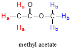
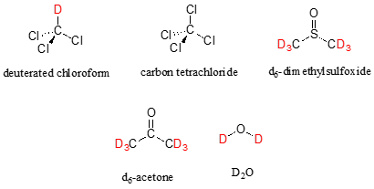
In most cases, a sample being analyzed by NMR is in solution. If we use a common laboratory solvent (diethyl ether, acetone, dichloromethane, ethanol, water, etc.) to dissolve our NMR sample, however, we run into a problem – there many more solvent protons in solution than there are sample protons, so the signals from the sample protons will be overwhelmed. To get around this problem, we use special NMR solvents in which all protons have been replaced by deuterium. Deuterium is NMR-active, but its resonance frequency is far outside of the range in which protons absorb, so it is `invisible` in ¹H-NMR. Some common NMR solvents are shown below.

Common NMR solvents

Note that this is not necessarily a problem when looking at nuclei such as ³¹P. Very few solvents contain phosphorus so there is no chance for the phosphorus signals to be overwhelmed by signals from the solvent. However, most spectra are still obtained in deuterated solvents because the instruments often rely on a deutrerium signal to fine tune the signal and a proton spectrum is often obtained along with spectra for other nuclei.

It should also be noted that when conducting an NMR experiment, the operator chooses which nucleus is being observed. As mentioned previously, the resonance frequency of deuterium is significantly different than that of protons. One could choose to observe a proton spectrum of a sample or the deuterium spectrum of the same sample, but not both at the same time. There are some very specialized experiments that do allow the observation of two different nuclei in the same experiment, but that is beyond the score of this course. If the ³¹P spectrum of a sample is obtained, the presence of protons in the solvent will not have an impact on the spectrum. This does not mean that different nuclei (e.g. phosphorus and proton) do not influence each other as we will see when we discuss coupling.

Let's look at an actual ¹H-NMR spectrum for methyl acetate. The vertical axis corresponds to intensity of absorbance, the horizontal axis to frequency. However, you will notice right away that a) there is no y-axis line or units drawn in the figure, and b) the x-axis units are not Hz, which you would expect for a frequency scale. Both of these mysteries will become clear very soon.

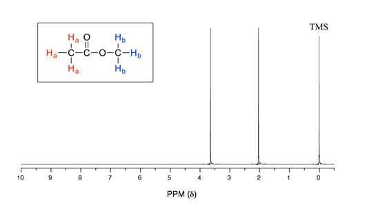
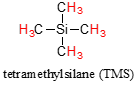
We see three absorbance signals: two of these correspond to H_a and H_b (don't worry yet which is which), while the peak at the far right of the spectrum corresponds to the 12 chemically equivalent protons in tetramethylsilane (TMS), a standard reference compound that was added to our sample.

First, let's talk about the x-axis. The 'ppm' label stands for 'parts per million', and simply tells us that the two sets of equivalent protons in our methyl acetate sample have resonance frequencies about 2.0 and 3.6 parts per million higher than the resonance frequency of the TMS protons, which we are using as our reference standard. This is referred to as their chemical shift.

The reason for using a relative value (chemical shift expressed in ppm) rather than the actual resonance frequency (expressed in Hz) is that every NMR instrument will have a different magnetic field strength, so the actual value of resonance frequencies expressed in Hz will be different on different instruments - remember that ΔE for the magnetic transition of a nucleus depends upon the strength of the externally applied magnetic field. However, the resonance frequency values relative to the TMS standard will always be the same, regardless of the strength of the applied field. For example, if the resonance frequency for the TMS protons in a given NMR instrument is exactly 300 MHz (300 million Hz), then a chemical shift of 2.0 ppm corresponds to an actual resonance frequency of 300,000,600 Hz (2 parts per million of 300 million is 600). In another instrument (with a stronger magnet) where the resonance frequency for TMS protons is 400 MHz, a chemical shift of 2.0 ppm corresponds to a resonance frequency of 400,000,800 Hz.

A frequently used symbolic designation for chemical shift in ppm is the lower-case Greek letter δ. Most protons in organic compounds have chemical shift values between 0 and 10 ppm relative to TMS, although values below 0 ppm and up to 12 ppm and above are occasionally observed. By convention, the left-hand side of an NMR spectrum (higher chemical shift) is called downfield, and the right-hand direction is called upfield.

In modern research-grade NMR instruments, it is no longer necessary to actually add TMS to the sample: the computer simply calculates where the TMS signal should be, based on resonance frequencies of the solvent. So, from now on you will not see a TMS peak on NMR spectra - but the 0 ppm point on the x-axis will always be defined as the resonance frequency of TMS protons.

A Chemical Shift Analogy

If you are having trouble understanding the concept of chemical shift and why it is used in NMR, try this analogy: imagine that you have a job where you travel frequently to various planets, each of which has a different gravitational field strength. Although your body mass remains constant, your measured weight is variable - the same scale may show that you weigh 60 kg on one planet, and 75 kg on another. You want to be able to keep track your body mass in a meaningful, reproducible way, so you choose an object to use as a standard: a heavy iron bar, for example. You record the weight of the iron bar and yourself on your home planet, and find that the iron bar weighs 50 kg and you weigh 60 kg. You are 20 percent (or pph, parts per hundred) heavier than the bar. The next day you travel (with the iron bar in your suitcase) to another planet and find that the bar weighs 62.5 kg, and you weigh 75 kg. Although your measured weight is different, you are still 20% heavier than the bar: you have a 'weight shift' of 20 pph relative to the iron bar, no matter what planet you are on.

We have already pointed out that, on our spectrum of methyl acetate, there is there is no y-axis scale indicated. With y-axis data it is relative values, rather than absolute values, that are important in NMR. The computer in an NMR instrument can be instructed to mathematically integrate the area under a signal or group of signals. The signal integration process is very useful, because in ¹H-NMR spectroscopy the area under a signal is proportional to the number of protons to which the signal corresponds. When we instruct the computer to integrate the areas under the H_a and H_b signals in our methyl acetate spectrum, we find that they have approximately the same area. This makes sense, because each signal corresponds to a set of three equivalent protons.

Be careful not to assume that you can correlate apparent peak height to number of protons - depending on the spectrum, relative peak heights will not always be the same as relative peak areas, and it is the relative areas that are meaningful. Because it is difficult to compare relative peak area by eye, we rely on the instrument's computer to do the calculations. Note also that in the spectrum above the signal for TMS represents 12 protons and yet is appears to be similar to the signals for the methyl acetate. The intensity of the signals is also dependent on the concentration of the species in solution. Without careful sample preparation, it is extremely unlikely that the concentration of TMS is the same as that of the methyl acetate meaning that there can not be a direct comparison of their signals.

Take a look next at the spectrum of 1,4-dimethylbenzene:

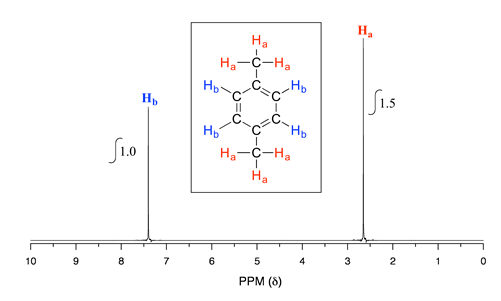
As we discussed earlier, this molecule has two sets of equivalent protons: the six methyl H_a protons and the four aromatic H_b protons. When we instruct the instrument to integrate the areas under the two signals, we find that the area under the peak at 2.6 ppm is 1.5 times greater than the area under the peak at 7.4 ppm. The ratio 1.5 to 1 is of course the same as the ratio 6 to 4. This integration information (along with the actual chemical shift values, which we'll discuss soon) tells us that the peak at 7.4 ppm must correspond to H_b, and the peak at 2.6 ppm to H_a.

Contributors

• Organic Chemistry With a Biological Emphasis by Tim Soderberg (University of Minnesota, Morris)