2.6: The Range of Bonding

In general chemistry we learned that bonding between atoms can classified as range of possible bonding between ionic bonds (fully charge transfer) and covalent bonds (fully shared electrons). When two atoms of slightly differing electronegativities come together to form a covalent bond, one atom attracts the electrons more than the other; this is called a polar covalent bond. However, simple “ionic” and “covalent” bonding are idealized concepts and most bonds exist on a two-dimensional continuum described by the van Arkel-Ketelaar Triangle (Figure \(\PageIndex{1}\)).

Figure \(\PageIndex{1}\): van Arkel-Ketelaar Triangle plots the difference in electronegativity (\(\Delta \chi\)) and the average electronegativity in a bond (\(\sum \chi\)). the top region is where bonds are mostly ionic, the lower left region is where bonding is metallic, and the lower right region is where the bonding is covalent.

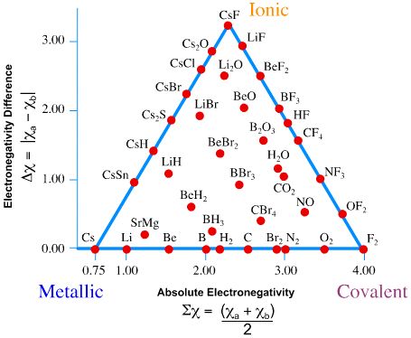
Bond triangles or van Arkel–Ketelaar triangles (named after Anton Eduard van Arkel and J. A. A. Ketelaar) are triangles used for showing different compounds in varying degrees of ionic, metallic and covalent bonding. In 1941 van Arkel recognized three extreme materials and associated bonding types. Using 36 main group elements, such as metals, metalloids and non-metals, he placed ionic, metallic and covalent bonds on the corners of an equilateral triangle, as well as suggested intermediate species. The bond triangle shows that chemical bonds are not just particular bonds of a specific type. Rather, bond types are interconnected and different compounds have varying degrees of different bonding character (for example, polar covalent bonds).

Video \(\PageIndex{1}\): What is the van Arkel-Ketelaar Triangle of Bonding?

Using electronegativity - two compound average electronegativity on x-axis of Figure \(\PageIndex{1}\).

\[\sum \chi = \dfrac{\chi_A + \chi_B}{2} \label{sum}\]

and electronegativity difference on y-axis,

\[\Delta \chi = | \chi_A - \chi_B | \label{diff}\]

we can rate the dominant bond between the compounds. On the right side of Figure \(\PageIndex{1}\) (from ionic to covalent) should be compounds with varying difference in electronegativity. The compounds with equal electronegativity, such as \(\ce{Cl2}\) (chlorine) are placed in the covalent corner, while the ionic corner has compounds with large electronegativity difference, such as \(\ce{NaCl}\) (table salt). The bottom side (from metallic to covalent) contains compounds with varying degree of directionality in the bond. At one extreme is metallic bonds with delocalized bonding and at the other are covalent bonds in which the orbitals overlap in a particular direction. The left side (from ionic to metallic) is meant for delocalized bonds with varying electronegativity difference.

The Three Extremes in bonding

In general:

• Metallic bonds have low \(\Delta \chi\) and low average \(\sum\chi\).
• Ionic bonds have moderate-to-high \(\Delta \chi\) and moderate values of average \(\sum \chi\).
• Covalent bonds have moderate to high average \(\sum \chi\) and can exist with moderately low \(\Delta \chi\).

Example \(\PageIndex{1}\)

Use the tables of electronegativities and Figure \(\PageIndex{1}\) to estimate the following values

• difference in electronegativity (\(\Delta \chi\))
• average electronegativity in a bond (\(\sum \chi\))
• percent ionic character
• likely bond type

for the selected compounds:

1. \(\ce{AsH}\) (e.g., in arsine \(AsH\))
2. \(\ce{SrLi}\)
3. \(\ce{KF}\).

Solution

a: \(\ce{AsH}\)

• The electronegativity of \(\ce{As}\) is 2.18
• The electronegativity of \(\ce{H}\) is 2.22

Using Equations \ref{sum} and \ref{diff}:

\[\begin{align*} \sum \chi &= \dfrac{\chi_A + \chi_B}{2} \\[4pt] &=\dfrac{2.18 + 2.22}{2} \\[4pt] &= 2.2 \end{align*}\]

\[\begin{align*} \Delta \chi &= \chi_A - \chi_B \\[4pt] &= 2.18 - 2.22 \\[4pt] &= 0.04 \end{align*}\]

• From Figure \(\PageIndex{1}\), the bond is fairly nonpolar and has a low ionic character (10% or less)
• The bonding is in the middle of a covalent bond and a metallic bond

b: \(\ce{SrLi}\)

• The electronegativity of \(\ce{Sr}\) is 0.95
• The electronegativity of \(\ce{Li}\) is 0.98

Using Equations \ref{sum} and \ref{diff}:

\[\begin{align*} \sum \chi &= \dfrac{\chi_A + \chi_B}{2} \\[4pt] &=\dfrac{0.95 + 0.98}{2} \\[4pt] &= 0.965 \end{align*}\]

\[\begin{align*} \Delta \chi &= \chi_A - \chi_B \\[4pt] &= 0.98 - 0.95 \\[4pt] &= 0.025 \end{align*}\]

• From Figure \(\PageIndex{1}\), the bond is fairly nonpolar and has a low ionic character (~3% or less)
• The bonding is likely metallic.

c: \(\ce{KF}\)

• The electronegativity of \(\ce{K}\) is 0.82
• The electronegativity of \(\ce{F}\) is 3.98

Using Equations \ref{sum} and \ref{diff}:

\[\begin{align*} \sum \chi &= \dfrac{\chi_A + \chi_B}{2} \\[4pt] &=\dfrac{0.82 + 3.98}{2} \\[4pt] &= 2.4 \end{align*}\]

\[\begin{align*} \Delta \chi &= \chi_A - \chi_B \\[4pt] &= | 0.82 - 3.98 | \\[4pt] &= 3.16 \end{align*}\]

• From Figure \(\PageIndex{1}\), the bond is fairly polar and has a high ionic character (~75%)
• The bonding is likely ionic.

Exercise \(\PageIndex{1}\)

Contrast the bonding of \(\ce{NaCl}\) and silicon tetrafluoride.

Answer

\(\ce{NaCl}\) is an ionic crystal structure, and an electrolyte when dissolved in water; \(\Delta \chi =1.58\), average \(\sum \chi =1.79\), while silicon tetrafluoride is covalent (molecular, non-polar gas; \(\Delta \chi =2.08\), average \(\sum \chi =2.94\).

Contributors and Attributions

• Jim Clark (Chemguide.co.uk)

• Daniel James Berger
• Wikipedia

• Ed Vitz (Kutztown University), John W. Moore (UW-Madison), Justin Shorb (Hope College), Xavier Prat-Resina (University of Minnesota Rochester), Tim Wendorff, and Adam Hahn.