2.2: Connection Tables

Learning Objectives:

• Introduce concept of Connection Table
• Introduce shortcomings of Simplified Connection Table

Introduction

A connection table is a data table that provides information a computer needs to generate a molecular graph. Specifically, it needs to define what the atoms are, and how they are connected, that is, the edges and the nodes of the graph. This is typically done in a file, and in the file are a minimum of two tables, the atom table and the bond table. But the file can also have additional information, like what isotopes are present, or what are the 3-D coordinates for a particular conformation.

Thus, this section will be broken up into several parts. First, we will discuss a Simplified Connection Table (SCT) to get a feel for the basic logic behind a connection table. Then we will look at some real files that students will be required to download from databases and work with.

Simplified Connection Table (SCT)

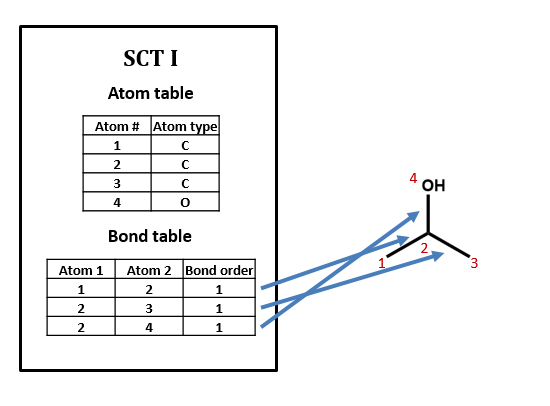
The purpose of this section is to give the student a feel for the issues associated with creating a connection table that can generate a molecular graph. The SCT is not a real file, but a description of the data within a file that the computer needs to be able to "read". Real files using connection tables will be approached in section 2.5 Structural Data Files. In essence, there are two tables, the atom table and the bond table.

• The atom table provides an index number for each atom. It may provide index numbers for the hydrogen (explicit representations), or it may not (implicit representations).
• The bond table uses the index number of the atom table to define what atoms are bonded to each other, and the types of bonds. The bond order is defined by a number, where 1 is a single bond, 2 is a double bond and 3 is a triple bond.

Figure \(\PageIndex{1}\): SCT for isopropanol.

Are connection tables unique?

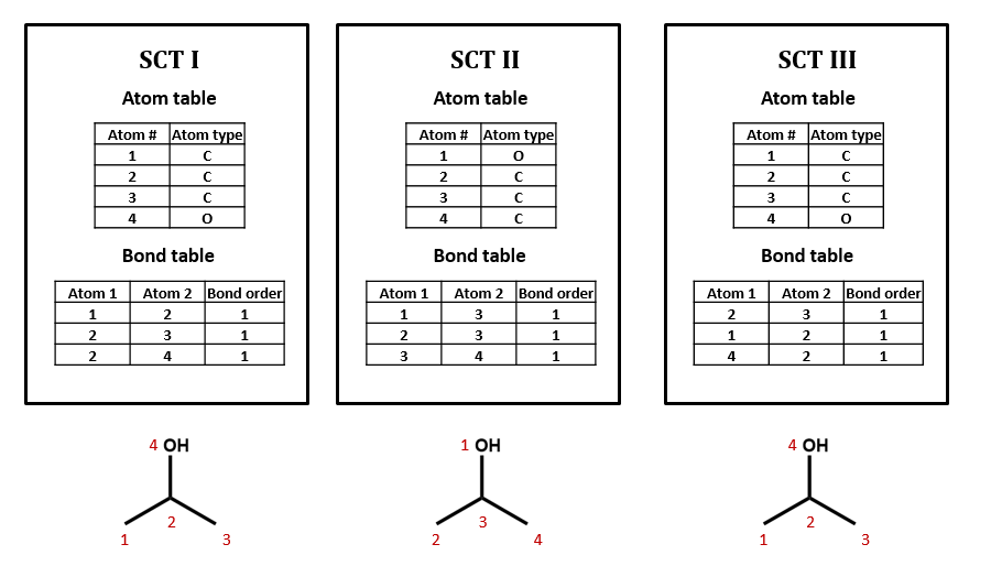
No, there can be many ways of assigning index numbers to the atoms in a connection table, and one would need to use an algorithm for generating a canonical connection table. For n atoms there are n! (n factorial) ways of assigning index numbers. From figure 2.2.2, if any of the four atoms is assigned the value of 1, there are 6 ways you can assign the remaining three atoms, and since there are 4 atoms you can assign the value of 1 to, there are 24 ways to assign the above index numbers, which is 4!.

Figure \(\PageIndex{2}\): Three possible ways of assigning index numbers to a connection table for isopropanol.

Was the above connection table explicit or implicit in the assignment of hydrogens?

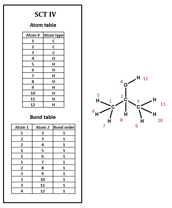
The above connection table is implicit in the assignment of hydrogens, and algorithms based on a set of valency rules could determine the number of hydrogens. Figure 2.2.3 has explicit hydrogens for isopropanol.

Figure \(\PageIndex{3}\): Isopropanol connection table with explicit hydrogens. 

By comparing figures 2.2.2 and 2.2.3 you can see how the implicit table is simpler and would result in a smaller file.

Exercise \(\PageIndex{1}\)

Can you see what is wrong with the Bond table in figure \(\PageIndex{3}\)?

Answer

Note that atom 2 is only in three bonds, and atom three is in five bonds, and that somehow, atom 3 is attached to atom 1.

SCT Shortcomings

The Simplified Connection Table is at the core of graph theory representation of chemical entities in that it provides the critical information of what atoms are present and where the bonds are. In section 2.5 we will look at several structural data files that are built around connection tables, but before that it is prudent to identify many of the issues with molecular representation that a crude SCT does not cover, and these will be outlined in section 2.3. There are sort of three basic types of shortcomings to connection tables.

The first is that real molecules are dynamic 3 dimensional structures and so a real data file needs to define the relative coordinates of the atoms, which is typically done by adding a 3D coordinate layer to the atom table (section 2.5). The fact that molecules are dynamic means the bonds are both vibrating and rotating, with the later resulting in multiple conformations (different orientations) of the atoms over time. Atomic coordinates typically represent the most stable orientation as determined through computational calculations that minimize the energy of the system and take into account environmental factors. This means the coordinates of a molecule in free space may be completely different than in a protein environment, and so it is important that you understand how the coordinates in a molecular data file were generated, and if they are appropriate to your needs.

The second shortcoming to connection tables is actually structural in nature, and often a SCT does not provide enough information to uniquely describe a molecular species. In the case of isopropanol above, there were 24 connection tables that described the molecule, but they all described the same molecule, that is, they described isoproponal. Sterioisomerism is a case where two different molecules (say cis and trans dichlorethene) would have the same connection table, and so stereo isomers would require additional information to uniquely distinguish between the two isomers. Other areas where issues with SCT arise include resonance structures, aromaticity, tautomers, multcovalent units, coordination complexes, conjugate acid/base equilibrium and the like. To handle these issues additional data beyond that of the SCT. These will be discussed in section 2.3 Molecular Graph Issues.

The third potential issue with connection table based representation of chemicals is more functional in nature, in that they are bulky files and hard to read by a human. Line notation is a string of characters, like a word, which describes the molecule. One could consider line notation to be nomenclature for computers in the sense that a string of characters represents a :word". In reality, line notations are often converted to connection tables when software agents are doing calculations because many of the software algorithms are based on manipulating connection tables.

The shortcomings of connection tables will be picked up again when we look at real structural data files and how they handle these situations.

Contributors

Robert E. Belford (University of Arkansas Little Rock; Department of Chemistry). The breadth, depth and veracity of this work is the responsibility of Robert E. Belford, [e-mail]. You should contact him if you have any concerns. This material has both original contributions, and content built upon prior contributions of the LibreTexts Community and other resources, including but not limited to:

• Evan Hepler-Smith
• Leah McEwen

(Material adopted from the Spring 2017 Cheminformatics OLCC)