2.1: Introduction
- Page ID
- 154255
\( \newcommand{\vecs}[1]{\overset { \scriptstyle \rightharpoonup} {\mathbf{#1}} } \)
\( \newcommand{\vecd}[1]{\overset{-\!-\!\rightharpoonup}{\vphantom{a}\smash {#1}}} \)
\( \newcommand{\dsum}{\displaystyle\sum\limits} \)
\( \newcommand{\dint}{\displaystyle\int\limits} \)
\( \newcommand{\dlim}{\displaystyle\lim\limits} \)
\( \newcommand{\id}{\mathrm{id}}\) \( \newcommand{\Span}{\mathrm{span}}\)
( \newcommand{\kernel}{\mathrm{null}\,}\) \( \newcommand{\range}{\mathrm{range}\,}\)
\( \newcommand{\RealPart}{\mathrm{Re}}\) \( \newcommand{\ImaginaryPart}{\mathrm{Im}}\)
\( \newcommand{\Argument}{\mathrm{Arg}}\) \( \newcommand{\norm}[1]{\| #1 \|}\)
\( \newcommand{\inner}[2]{\langle #1, #2 \rangle}\)
\( \newcommand{\Span}{\mathrm{span}}\)
\( \newcommand{\id}{\mathrm{id}}\)
\( \newcommand{\Span}{\mathrm{span}}\)
\( \newcommand{\kernel}{\mathrm{null}\,}\)
\( \newcommand{\range}{\mathrm{range}\,}\)
\( \newcommand{\RealPart}{\mathrm{Re}}\)
\( \newcommand{\ImaginaryPart}{\mathrm{Im}}\)
\( \newcommand{\Argument}{\mathrm{Arg}}\)
\( \newcommand{\norm}[1]{\| #1 \|}\)
\( \newcommand{\inner}[2]{\langle #1, #2 \rangle}\)
\( \newcommand{\Span}{\mathrm{span}}\) \( \newcommand{\AA}{\unicode[.8,0]{x212B}}\)
\( \newcommand{\vectorA}[1]{\vec{#1}} % arrow\)
\( \newcommand{\vectorAt}[1]{\vec{\text{#1}}} % arrow\)
\( \newcommand{\vectorB}[1]{\overset { \scriptstyle \rightharpoonup} {\mathbf{#1}} } \)
\( \newcommand{\vectorC}[1]{\textbf{#1}} \)
\( \newcommand{\vectorD}[1]{\overrightarrow{#1}} \)
\( \newcommand{\vectorDt}[1]{\overrightarrow{\text{#1}}} \)
\( \newcommand{\vectE}[1]{\overset{-\!-\!\rightharpoonup}{\vphantom{a}\smash{\mathbf {#1}}}} \)
\( \newcommand{\vecs}[1]{\overset { \scriptstyle \rightharpoonup} {\mathbf{#1}} } \)
\(\newcommand{\longvect}{\overrightarrow}\)
\( \newcommand{\vecd}[1]{\overset{-\!-\!\rightharpoonup}{\vphantom{a}\smash {#1}}} \)
\(\newcommand{\avec}{\mathbf a}\) \(\newcommand{\bvec}{\mathbf b}\) \(\newcommand{\cvec}{\mathbf c}\) \(\newcommand{\dvec}{\mathbf d}\) \(\newcommand{\dtil}{\widetilde{\mathbf d}}\) \(\newcommand{\evec}{\mathbf e}\) \(\newcommand{\fvec}{\mathbf f}\) \(\newcommand{\nvec}{\mathbf n}\) \(\newcommand{\pvec}{\mathbf p}\) \(\newcommand{\qvec}{\mathbf q}\) \(\newcommand{\svec}{\mathbf s}\) \(\newcommand{\tvec}{\mathbf t}\) \(\newcommand{\uvec}{\mathbf u}\) \(\newcommand{\vvec}{\mathbf v}\) \(\newcommand{\wvec}{\mathbf w}\) \(\newcommand{\xvec}{\mathbf x}\) \(\newcommand{\yvec}{\mathbf y}\) \(\newcommand{\zvec}{\mathbf z}\) \(\newcommand{\rvec}{\mathbf r}\) \(\newcommand{\mvec}{\mathbf m}\) \(\newcommand{\zerovec}{\mathbf 0}\) \(\newcommand{\onevec}{\mathbf 1}\) \(\newcommand{\real}{\mathbb R}\) \(\newcommand{\twovec}[2]{\left[\begin{array}{r}#1 \\ #2 \end{array}\right]}\) \(\newcommand{\ctwovec}[2]{\left[\begin{array}{c}#1 \\ #2 \end{array}\right]}\) \(\newcommand{\threevec}[3]{\left[\begin{array}{r}#1 \\ #2 \\ #3 \end{array}\right]}\) \(\newcommand{\cthreevec}[3]{\left[\begin{array}{c}#1 \\ #2 \\ #3 \end{array}\right]}\) \(\newcommand{\fourvec}[4]{\left[\begin{array}{r}#1 \\ #2 \\ #3 \\ #4 \end{array}\right]}\) \(\newcommand{\cfourvec}[4]{\left[\begin{array}{c}#1 \\ #2 \\ #3 \\ #4 \end{array}\right]}\) \(\newcommand{\fivevec}[5]{\left[\begin{array}{r}#1 \\ #2 \\ #3 \\ #4 \\ #5 \\ \end{array}\right]}\) \(\newcommand{\cfivevec}[5]{\left[\begin{array}{c}#1 \\ #2 \\ #3 \\ #4 \\ #5 \\ \end{array}\right]}\) \(\newcommand{\mattwo}[4]{\left[\begin{array}{rr}#1 \amp #2 \\ #3 \amp #4 \\ \end{array}\right]}\) \(\newcommand{\laspan}[1]{\text{Span}\{#1\}}\) \(\newcommand{\bcal}{\cal B}\) \(\newcommand{\ccal}{\cal C}\) \(\newcommand{\scal}{\cal S}\) \(\newcommand{\wcal}{\cal W}\) \(\newcommand{\ecal}{\cal E}\) \(\newcommand{\coords}[2]{\left\{#1\right\}_{#2}}\) \(\newcommand{\gray}[1]{\color{gray}{#1}}\) \(\newcommand{\lgray}[1]{\color{lightgray}{#1}}\) \(\newcommand{\rank}{\operatorname{rank}}\) \(\newcommand{\row}{\text{Row}}\) \(\newcommand{\col}{\text{Col}}\) \(\renewcommand{\row}{\text{Row}}\) \(\newcommand{\nul}{\text{Nul}}\) \(\newcommand{\var}{\text{Var}}\) \(\newcommand{\corr}{\text{corr}}\) \(\newcommand{\len}[1]{\left|#1\right|}\) \(\newcommand{\bbar}{\overline{\bvec}}\) \(\newcommand{\bhat}{\widehat{\bvec}}\) \(\newcommand{\bperp}{\bvec^\perp}\) \(\newcommand{\xhat}{\widehat{\xvec}}\) \(\newcommand{\vhat}{\widehat{\vvec}}\) \(\newcommand{\uhat}{\widehat{\uvec}}\) \(\newcommand{\what}{\widehat{\wvec}}\) \(\newcommand{\Sighat}{\widehat{\Sigma}}\) \(\newcommand{\lt}{<}\) \(\newcommand{\gt}{>}\) \(\newcommand{\amp}{&}\) \(\definecolor{fillinmathshade}{gray}{0.9}\)- Gain understanding of chemical structural data
- Introduce basic ways of communicating structural data
Representing Chemicals
In your studies of chemistry starting in the freshmen years you have encountered many ways of representing chemicals, and here we will list a few.
- Trivial Names (Aspirin)
- Systematic Names (2-acetyloxybenzoic acid)
- Formula (C9H8O4)
- Images
We will now look at several other ways of representing chemicals, most notably connection tables and line notation.
Chemical Representation for Cheminformatics
Most often, data and information about chemical compounds is either directly about molecular structure (for example, a 2D structural formula, or 3D atomic coordinates for a particular conformation of a compound), or is tied to a molecular structure (for example, physical properties of a compound, which you identify by its structural formula). The notion of indexing, sorting, searching and retrieving information using molecular structures originated within the domain of modern chemistry.
Almost all chemists engage in communication tasks to register, search, view, and publish molecular structures. Most forms of chemical representation were developed with these uses in mind. Cheminformatics involves storing, finding, and analyzing these structures using the data-processing power of computers to match chemical compounds with literature publications, measured properties, synthetic procedures, spectra, and computational studies. To do this work, computers need to use chemical representation to identify, exchange and validate information about chemical compounds.
In order for (human) chemists to rely on insights from cheminformatics, it is important to understand the way in which computers store and analyze chemical structure, the methods that computer programs employ, and the results that they produce. Therefore, cheminformatics depends upon the use of representations of molecular structures and related data that are understandable both to human scientists and to machine algorithms.
Formulating Chemical Structure Data
Interacting with a machine is a form of communication. How does communication between chemists differ from communication between a chemist and a machine? In cheminformatics, you are working within a system governed by strict rules that are explicitly defined. If you know the rules, then you can make the system work for you. If you don't know the rules for a given form of representation, sometimes features designed to satisfy the requirements in one context will appear as bugs in another context.
If one chemist was to recommend to another that a reaction should be performed using "chloroform" as a solvent for a reaction, this would generally be a successful exercise in communication. For all practical purposes, this word is understood by every chemist, and has no ambiguity. However, because "chloroform" is a so-called trivial name, there is no formula for converting it into the actual chemical structure that it represents, and a machine will not be able to participate in this exchange of information unless it has been explicitly instructed as to the chemical structure that this word represents, expressed in a format that the machine can work with.
A more descriptive way to communicate the composition that is chloroform is by chemical formula, in this case CHCl3. A computer program could interpret basic molecular structure rules to determine that the substance being described has 5 atoms: 1 carbon, 1 hydrogen and 3 chlorine. Assembling this into a molecule with bonds can be based on valence rules, identifying 4 of the atoms as normally monovalent and one as normally tetravalent. It is quite simple to create a software algorithm that can join the atoms together in the most obvious way, which also happens to be correct.
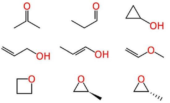
Beyond such tiny simple molecules, difficulties soon arise. Some of these ambiguities affect human chemists in the same way that they affect machines. Consider the molecular formula of C3H6O, which is associated with multiple reasonable structures, including a ketone, an aldehyde, a cyclic alcohol, oxygenated alkenes and cyclic ethers, one of which exists as two enantiomers:

Figure \(\PageIndex{1}\): Different ways of drawing C3H6O (Image credit: Evan Hepler-Smith)
Ambiguous representations can refer to more than one chemical entity. This is true of most chemical names when used unsystematically, such as “octane,” when employed as a common term for all saturated hydrocarbons with eight carbon atoms, rather than systematically to indicate the straight-chain isomer only. Empirical and molecular formulas are also typically ambiguous.
In an unambiguous system of representation, each name or formula refers to exactly one chemical entity, typically in a way that allows you to draw a structural formula for it. However, each chemical entity might be represented by more than one name or formula. A canonical form is a completely unique representation within a system. For example, “diethyl ketone” and “3-pentanone” are both unambiguous names: each represents one and only one compound. However, since they represent the same compound, they are not unique names. Within the system of Preferred IUPAC Names (see below), “3-pentanone” is a canonical name – an unambiguous and unique representation of this compound.
Note that, since canonical names are necessarily canonical within a system, they might not function properly if you are interested in structural information that is not addressed within the system, or if you do not have structural information that is required by the system. For example, within a system that does not address stereochemistry, the different enantiomers of a chiral compound will have the same “canonical” representation. Within a system that requires the specification of stereochemistry, on the other hand, you will have to choose between stereospecific canonical representations. If you happen to be working with a racemic mixture or a compound of unknown stereo configuration, this may lead to misrepresentation and misunderstanding.
A chemical structure representation contains two kinds of information: explicit and implicit. Explicit information is what’s directly represented in a data structure and should at minimum contain what otherwise would not be known, such as the specific atom in a carbon skeleton to which a substituent is attached. Implicit information is what you (or a computer) can figure out from a data structure, given some knowledge of general principles and a little bit of work.
In general, data structures that contain less explicit information are more simple and compact, but they require more computation to draw chemical conclusions from them. Data structures that contain more explicit information take up more space and are at greater risk of containing inconsistencies, but they can be more quickly analyzed in a wider variety of ways.
To automate functions on chemical data, the data structure needs to be systematically defined and consistently applied. These definitions are part of what constitutes explicit information that an algorithm can readily identify and parse. Balancing the level of explicit information can also impact the ambiguity of a system, and the ability to accurately exchange chemical structures between systems. These are especially important considerations for operations that range across a significant portion of the corpus of reported chemical compounds (well over 100 million), beyond the scale at which human validation of results is possible.
Representing Chemical Structure
Structural Formula
Generally, the most effective way to communicate with another chemist about the structure of a compound is to draw its structural formula. A structural formula is any formula that indicates the connectivity of a compound – that is, which of its atoms are linked to each other by covalent bonds. Unfortunately, structural formula are most valuable for small molecules as they can get to complex as the size of the molecule increases. On the other hand, a computer does not "see" a formula like a human does, but "reads" it as a form of data, and we will look at two data structures that computers can "read", connection tables and line notations.
Systematic Names
Systematic names describe the structural formula of compounds. If you know the rules and vocabulary, you should be able to write a name based on a structural formula and vice-versa. Chemists have developed various ways of translating formulas into names, so it is nearly always possible to write more than one systematic name for a given compound.
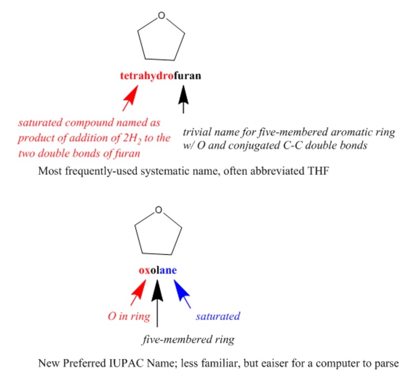
IUPAC (International Union of Pure and Applied Chemistry) nomenclature is a well-known international system of chemical names that is generally systematic but flexible, allowing the use of certain well-established trivial names. Since systematic IUPAC names are made according to formalized rules, they could, in principle, be used by both humans and computers. However, IUPAC names are often quite difficult for chemists to read, let alone to write, and the rules are non-canonical, resulting in numerous different options for naming each compound. IUPAC has introduced even more rules for determining canonical Preferred IUPAC Names (PINs) that are oriented toward making systematic names more easily readable by machines.

Semantic technologies further enable systematic classification and organization of scientific terms, including descriptions of chemical structures, such as provided by ChEBI (Chemical Entities of Biological Interest). ChEBI describes small molecular entities based on nomenclature, symbolism and terminology endorsed by IUPAC and the Nomenclature Committee of the International Union of Biochemistry and Molecular Biology (NC-IUBMB). This dataset is highly curated by both human experts and machine processes, is openly searchable and programmatically accessible, and includes full references to original authoritative sources.
Copyright Statement

The work in sections 1 & 2 above have been adopted or modified from original work of Evan Hepler-Smith and Leah McEwen from the 2017 Cheminformatics OLCC and is available here. This work is licensed under a Creative Commons Attribution-NonCommercial-Shar
Graphic Visualizations
Cheminformatics takes advantage of the mathematical discipline of graph theory when representing and comparing chemical structures. A graph represents the relationship between two things and graph theory involves the pair-wise relationship between two objects, where the object is a node (vertice or point on the graph) and the connection between the nodes are the edges (links or lines) of the graph. In chemistry the atoms are the vertices and the bonds are the edges. In fact you use graph theory when you use Google Maps to choose a route between two cities, where the cities are the vertices and the roads connecting them are the edges.
|
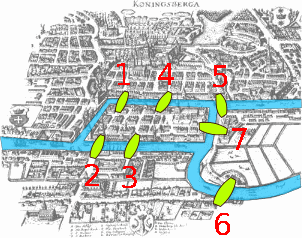
Konigsberg Bridges on map (credit: Maksim, Wikimedia Commons) |
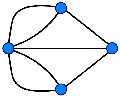
 Konigsberg Bridge Problem in terms of graph (credit: Riojajar, Wikimedia Commons) Konigsberg Bridge Problem in terms of graph (credit: Riojajar, Wikimedia Commons) |
(credit: Office of Naval Research, Technical Report No. 41, An introduction to Graph Theory, D.H. Rouvray) |
Figure \(\PageIndex{2}\): On the left is a map of Konigsberg (left), a graph describing the map (middle) and some simple molecules and their graphs (right).
In 1736 Leonhard Euler formulated the foundations of graph theory when he tackled the Konigsberg bridge problem, which was to determine if you could walk across every bridge to this island in the city of Knogsberg just once and walk across all of the bridges, (and he proved that you could not). Mathematically, Euler treated the land masses as the nodes and the bridges as the edges that link the nodes. In 1878 the mathematician James Sylvester introduced the concept of the chemicograph in his Journal of Nature article "Chemistry and Algebra", the same year he published the chemicographs of figure 3 in Volume 1, No. 1 of his American Journal of Mathematics article "On an Application of the New Atomic Theory to the Graphical Representation of the Invariants and Covariants of Binary Quantics, with Three Appendices". In Sylvester's chemicograph the atoms became the nodes and the covalent bonds the edges, and note, a double or triple bond were treated like having two or three edges connecting the nodes (atoms). One can quickly see a relationship between these and the Lewis Dot structures chemistry students cover in high school and freshmen chemistry, but as we shall see, computers can handle structures much more complicated than we can draw on a paper.
Figure \(\PageIndex{3}\): First eleven of forty five chemicographs from Sylvester's 1878 article on the Application of the New Atomic Theory to the Graphical Representation of the Invariants and Covariants of Binary Quantics, with Three Appendices".
One of the advantages to graph theory is it can be used to determine if two graphs have a one-to-one mapping of nodes and edges, that is if they are isomorphic (identical), and if a subgraph of one graph is isomorphic to a subgraph of another, those parts are identical. Although this elementary introductory course will not delve into graph theory, it is important that students understand the basic data structures that graph theory based algorithms use, and yes, we will be using those algorithms.
Chemical Graphs on Computers
Connection tables
A connection tables does for computers what systematic nomenclature does for human chemists: they organize structural information defined in a molecular graph in a form that is machine readable. The difference is that computers can read, sort, search, and group connection tables far faster than humans can work with systematic names or any other kind of formula or notation. Connection tables essentially provide information on the atoms in a molecule, where the bonds are, and what types of bonds there are. They are covered in more depth in section 2.2 and there are many types of structural data files that use connection tables (section 2.5). Besides connection tables, other common forms of machine-readable representations are graphic visualizations, line notations, and other descriptive forms such as nomenclature.
Chemists most frequently think about chemical structure in 2D, although molecules actually exist in 3D physical space. Most chemical data systems offer 2D and 3D visualizations that human chemists can use in searching and analysis. The 2D coordinates stored in a connection table can be used to infer and display chemical information, including the basic structural formula and additional information such as the E/Z geometry of alkene-like double bonds, the cis/trans isomerism of ligands in a square planar metal complex, or substituents on a cyclic alkane. 2D representations are designed to mimic the experience of drawing structural formulas on paper. Human often convert these electronic drawings two images files for use in publications and presentations, but these image files (jpeg, gif, ping,....) are no longer connected directly to chemical data and are thus not machine readable.
3D (x,y,z) coordinates can also be stored for each atom and used to display the conformation of a molecule. These coordinates may be determined experimentally (typically via x-ray crystallography), or calculated (using force-fields, quantum chemistry, molecular dynamics or composite models such as docking). Understanding a molecule's actual shape, whether it be in solution, in a vacuum, or in the binding site of a protein, opens up a whole new domain of computational chemistry. Most molecules have some flexibility, and even if a given conformation is the most stable, there are often a number of competing shapes to consider. Knowing how a particular set of coordinates was determined is crucial to making intelligent use of it for cheminformatics purposes.
Line Notations
Line notations represent chemical structures as a linear string of symbolic characters that can be interpreted by systematic rule sets and will be covered in section 2.3. Line notation could be considered as nomenclature for computers, as like a connection table a computer can "read" a line notation and develop a molecule the same way a human can read IUPAC nomenclature and generate the molecule. Many forms of line notation are both machine and human readable.
Line notation is widely used in Cheminformatics because:
- many computational processes operate more effectively on data structured as linear strings than data structured as tables.
- line notations can be reasonably legible to human chemists designing functions with these tools.
Linear representations are particularly well-suited to many identification and characterization functions, such as determining:
- whether molecules are the same;
- how similar they are, according to some metric;
- whether one molecular entity is a substructure of another;
- whether two molecules are related by a specific transformation;
- what happens when molecules are cut into pieces and grafted together at different positions.
In these and other applications of cheminformatics, linear line notation representations have key advantages for speed and automation, especially when you’d like to handle huge numbers of structures (e.g. searching a large database).
Examples of line notations include the Wiswesser Line-Formula Notation (WLN), Sybyl Line Notation (SLN) and Representation of structure diagram arranged linearly (ROSDAL). Currently, the most widely used linear notations are the Simplified Molecular-Input Line-Entry System (SMILES) and the IUPAC Chemical Identifier (InChI). In this class we will focus on SMILES and InChI line notation.
Contributors
Robert E. Belford (University of Arkansas Little Rock; Department of Chemistry). The breadth, depth and veracity of this work is the responsibility of Robert E. Belford, rebelford@ualr.edu. You should contact him if you have any concerns. This material has both original contributions, and content built upon prior contributions of the LibreTexts Community and other resources, including but not limited to:
- Evan Hepler-Smith
- Leah R. McEwen
- Acknowledgements: Alex Clark, Sunghwan Kim


