9.5: Ligand Field Theory

Extension of Crystal Field Theory

Experimentally it is known that the nature of the ligand plays an important role in the magnitude of the crystal field splitting in metal complexes and can determine whether a complex is high or low spin. Empirically ligands can be ordered in the spectrochemical series, but using crystal field theory we cannot rationalize where ligands fall in the series. For example, why is the neutral CO one of the strongest field ligands in the series while the anionic halogens are weak field ligands? To understand why ligands behave differently we have to consider how ligand orbitals interact with the metal d orbitals. Ligand field theory is essentially a combination between crystal field theory and molecular orbital theory where we focus only on the orbital overlap between the metal d orbitals and select ligand orbitals (rather than considering all of the valence orbitals on both the metal and ligand)

Metal-Ligand σ Bonding

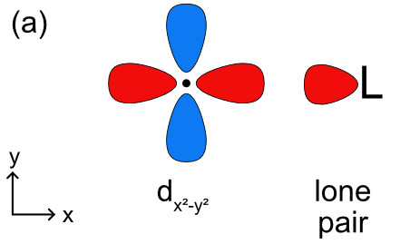
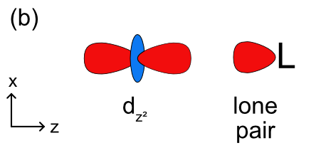
The bond between a metal and a ligand is primarily a Lewis acid-base interaction where the ligand is a Lewis base and donates a pair of electron to the metal, the Lewis acid. This interaction forms a coordinate covalent bond. As with molecular orbital theory we have to decide how (or if) the ligand lone pairs will overlap with each of the d orbitals, and what type of bonding will be formed In an octahedral complex the ligands and their lone pairs lie along the x, y, and z axes. As shown in Figure \(\PageIndex{1}\), the two on axis d orbitals (\(d_{x^2-y^2}\) and \(d_{z^2}\)) have to correct orientation to form sigma bonds with the ligands. With the three off axis d orbitals (\(d_{xy}\), \(d_{xz}\), and \(d_{yz}\)) the ligand lone pair overlaps with a node in these orbitals (Figure \(\PageIndex{1c}\)). This means there is no net overlap and no bonding (or antibonding) molecular orbital can be formed.

Figure \(\PageIndex{1a}\): Overlap between a ligand lone pair orbital and the metal \(d_{x^2-y^2}\) orbital to form a sigma bond (CC BY-NC-SA, Catherine McCusker)

Figure \(\PageIndex{1b}\): Overlap between a ligand lone pair orbital and the metal \(d_{z^2}\) orbital to form a sigma bond (CC BY-NC-SA, Catherine McCusker)

Figure \(\PageIndex{1c}\): There is no net overlap between the ligand lone pair orbital and the \(d_{xy}\) metal orbital, so this is a non bonding interaction (CC BY-NC-SA, Catherine McCusker)

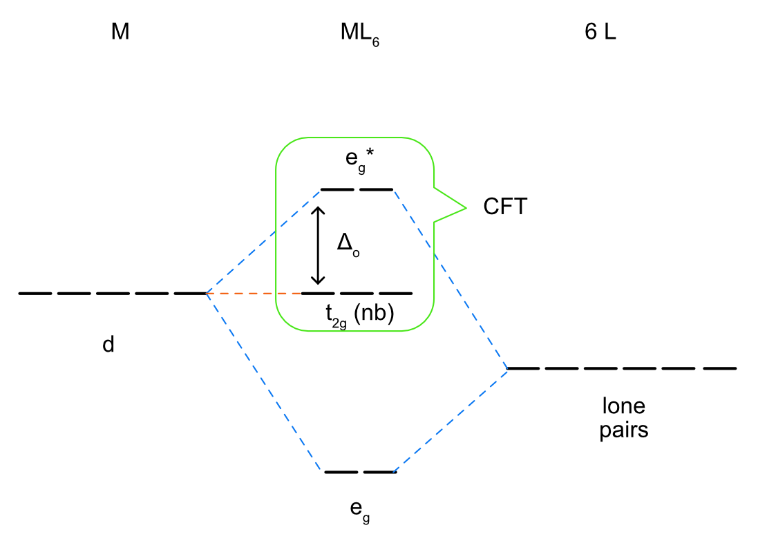
Knowing this, we can construct a ligand field splitting diagram (a simplified molecular orbital diagram) (Figure \(\PageIndex{2}\)). In the free metal ion all 5 of the d orbitals are degenerate and before they interact with the metal all 6 of the ligand lone pair orbitals are at the same energy as well. Generally, based on electronegativity the ligand lone pair orbitals will be lower in energy than the metal d orbitals. When the ligand lone pairs interact with metal d orbitals the on axis set of d orbitals (\(d_{x^2-y^2}\) and \(d_{z^2}\)) will form sigma bonding (e_g) and sigma antibonding (e_g*) molecular orbitals. The off axis set of d orbitals are nonbonding and are not stabilized or destabilized by the ligand lone pairs. Unlike a complete molecular orbital diagrams, a ligand field diagram won't necessarily have the same number of molecular orbitals as atomic orbitals becuse not every possible bonding interaction is included (for example, any overlap between the ligand orbitals and the metal s and p orbitals are not included). As in crystal field theory we can define an octahedral ligand field splitting energy (Δ_o), which will be the difference between the two molecular orbitals with the most metal d orbital character. In Figure \(\PageIndex{2}\) the t_2g set of d orbitals are nonbonding and therefore 100% metal character. The e_g bonding orbital is closer in energy to the ligand lone pairs and will have a higher % contribution from the ligands, and the e_g* antibonding orbital is closer in energy to the metal d orbitals and will have a higher % contribution from the metal. The relevant energy difference is between the t_2g and e_g* orbitals, as highlighted in green in Figure \(\PageIndex{2}\). The splitting energy will increase as there is a stronger interaction between the metal and ligand orbitals (based on the criteria discussed previously) and the e_g* is more destabilized.

Figure \(\PageIndex{2}\): Octahedral ligand field splitting diagram for only sigma bonding. The \(d_{x^2-y^2}\) and \(d_{z^2}\) metal orbitals form sigma bonding (e_g) and antibonding molecular orbitals (e_g*). The \(d_{xy}\), \(d_{xz}\), and \(d_{yz}\) orbital are nonbonding (t_2g (nb)). The green outline highlights the portion of the diagram that is equivalent to the crystal field splitting diagram. (CC BY-NC-SA; Catherine McCusker)

Metal-Ligand \(\pi\) Bonding

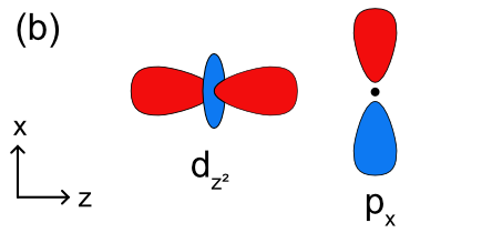
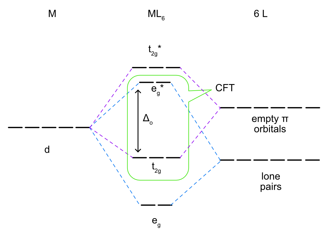
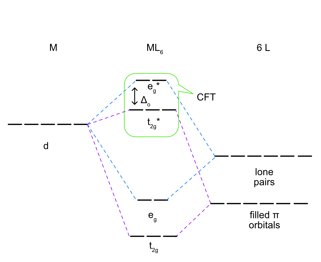
In addition to sigma bonding, some ligands have orbitals available which can form \(\pi\) bonds with metals as well. These could include p orbitals on a single donor atom such as a halogen ion or \(\pi\) bonding or antibonding molecular orbitals on a molecular ligand. To determine how \(\pi\) bonding will change the ligand field splitting picture in Figure \(\PageIndex{2}\), we will visualize how a ligand p orbital will interact with the metal d orbitals. The \(d_{x^2-y^2}\) and \(d_{z^2}\) orbitals do not have the correct symmetry to form any type of bond with a ligand p orbital as shown in Figures \(\PageIndex{3a-b}\) The \(d_{xy}\), \(d_{xz}\), and \(d_{yz}\) orbitals all have the correct symmetry to form \(\pi\) bonds with a ligand p orbital (Figure \(\PageIndex{3c}\)).

Figure \(\PageIndex{3a}\): There is no net overlap between the ligand p orbital and the \(d_{x^2-y^2}\) metal orbital, so this is a non bonding interaction (CC BY-NC-SA, Catherine McCusker)

Figure \(\PageIndex{3b}\): There is no net overlap between the ligand p orbital and the \(d_{z^2}\) metal orbital, so this is a non bonding interaction (CC BY-NC-SA, Catherine McCusker)

Figure \(\PageIndex{3c}\): Overlap between a ligand p orbital and the metal \(d_{xy}\) orbital to form a \(\pi\) bond (CC BY-NC-SA, Catherine McCusker)

Unlike metal-ligand \(\sigma\) bonding, where electrons are always donated from the ligand to the metal, electrons in metal-ligand \(\pi\) bonding can be donated from either the metal or the ligand depending on the nature of the orbitals involved. In cases where ligands have empty p or \(\pi\) symmetry orbitals that are close in energy to the metal d orbitals, they can accept electrons from a filled metal orbital. This is also known as \(\pi\) backbonding because the direction of electron donation is opposite of that found in sigma metal ligand bonding. These ligands are called \(\pi\) acceptor ligands. In cases where ligands have filled p or \(\pi\) symmetry orbitals that are close in energy to the metal d orbitals, they can donate electrons to an empty metal orbital. These ligands are called \(\pi\) donor ligands.

Figure \(\PageIndex{4}\): Illustration of metal-ligand \(\pi\) bonding with \(\pi\) acceptor and donor ligands. Filled orbitals are represented with black dots. (CC BY-NC-SA, Catherine McCusker)

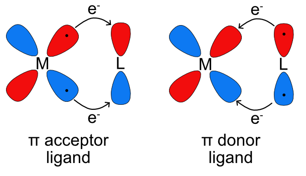
\(\pi\) Acceptors

Ligands that are \(\pi\) acceptors have empty, low energy \(\pi\) symmetry orbitals available to accept electrons from the metal center. Most often this is a \(\pi\)* antibonding molecular orbital but it could also be an empty p orbital. Due to the aufbau principle, these empty orbitals will be higher in energy than any filled lone pairs on the ligands and will also generally be higher energy than the metal d orbitals. Similar to multiple bonding in main group compounds \(\pi\) bonding always occurs in combination with sigma bonding so in the ligand field splitting diagram of metal-ligand bonding with a \(\pi\) acceptor ligand the lone pairs for sigma bonding must be included as well as the empty orbitals for \(\pi\) bonding. As seen in Figure \(\PageIndex{3}\), the \(d_{x^2-y^2}\) and \(d_{z^2}\) orbitals do not overlap with the ligand p orbitals. The on axis d orbitals will form sigma bonding (e_g) and sigma antibonding (e_g*) molecular orbitals. Unlike the sigma bonding only diagram, the off axis d orbitals (\(d_{xy}\), \(d_{xz}\), and \(d_{yz}\)) overlap with the ligand p orbitals to form \(\pi\) bonding (t_2g) and \(\pi\) antibonding (t_2g*) molecular orbitals as seen in Figure \(\PageIndex{5}\). Rather than being nonbonding, like in the sigma bonding only picture, the metal based t_2g molecular orbital is bonding. This increases the energy difference between the t_2g and e_g* and therefore increases Δ_o.

Figure \(\PageIndex{5}\): Octahedral ligand field splitting diagram with a \(\pi\) acceptor ligand. The \(d_{x^2-y^2}\) and \(d_{z^2}\) metal orbitals form sigma bonding (e_g) and antibonding molecular orbitals (e_g*) with the ligand lone pairs. The \(d_{xy}\), \(d_{xz}\), and \(d_{yz}\) orbital form pi bonding (t_2g) and pi antibonding molecular orbitals (t_2g*) with the empty \(\pi\) symmetry orbitals. The green outline highlights the portion of the diagram that is equivalent to the crystal field splitting diagram. (CC BY-NC-SA; Catherine McCusker)

Exercise \(\PageIndex{1}\)

Carbon monoxide is one of the most common, and strongest \(\pi\) acceptor ligands in inorganic chemistry. Refer to the molecular orbital diagram of CO and sketch likely metal-ligand orbital interactions for both sigma and pi bonding in a metal-CO complex. Indicate the direction of electron donation in both cases.

Answer

Sigma bonding:

Sigma bonding between a metal ion and a CO ligand involves overlap between the HOMO of CO (3σ) and the metal \(d_{x^2-y^2}\) or \(d_{z^2}\) orbitals. Electrons are donated from the ligand to the metal.

Pi bonding:

Pi bonding between a metal ion and CO ligand involves overlap between the LUMO of CO (\(\pi\)*) and the metal \(d_{xy}\), \(d_{xz}\), or \(d_{yz}\) orbitals. Electrons are donated from the metal to the ligand.

\(\pi\) Donor Ligands

Ligands that are \(\pi\) donors have filled \(\pi\) symmetry orbitals that are high enough in energy to donate electrons to the metal center. Most often this is a filled p orbital, but it could also be a \(\pi\) bonding molecular orbital. As lone pairs are generally the highest occupied orbitals is a molecule, the filled \(\pi\) orbitals will be lower in energy as seen in Figure \(\PageIndex{6}\). The sigma interaction between the ligand lone pairs and the metal \(d_{x^2-y^2}\) and \(d_{z^2}\) remain the same as previously described, forming the e_g bonding and e_g* antibonding molecular orbitals. The \(d_{xy}\), \(d_{xz}\), and \(d_{yz}\) overlap with the filled \(\pi\) orbitals to form \(\pi\) bonding (t_2g) and \(\pi\) antibonding (t_2g*) molecular orbitals. The difference between the \(pi\) acceptor and donor ligands is the energy and character of the t_2g and t_2g* molecular orbitals. In the \(\pi\) acceptor case above, the t_2g orbital is above the e_g and has a higher contribution from the metal and the t_2g* is above the e_g* and has a higher contribution from the ligand. In the \(\pi\) donor case the opposite is true. The t_2g orbital is below the e_g and has a higher contribution from the ligand and the t_2g* is below the e_g* and has a higher contribution from the metal. In this case Δ_o is smaller than in the sigma only picture because the t_2g symmetry molecular orbital has gone from nonbonding to antibonding and the energy difference between t_2g* and e_g* is smaller.

Figure \(\PageIndex{6}\): Octahedral ligand field splitting diagram with a \(\pi\) donor ligand. The \(d_{x^2-y^2}\) and \(d_{z^2}\) metal orbitals form sigma bonding (e_g) and antibonding molecular orbitals (e_g*) with the ligand lone pairs. The \(d_{xy}\), \(d_{xz}\), and \(d_{yz}\) orbital form pi bonding (t_2g) and pi antibonding molecular orbitals (t_2g*) with the filled \(\pi\) symmetry orbitals. The green outline highlights the portion of the diagram that is equivalent to the crystal field splitting diagram. (CC BY-NC-SA; Catherine McCusker)

The Spectrochemical Series

As discussed above, crystal field theory alone can't distinguish the behaviors of different ligands or explain why some ligands inherently produce larger splittings than others. Armed with ligand field theory we can now revisit the spectrochemical series and explain why ligands fall where they do within the series.

Strong field ligands

Strong field ligands are ones that produce large splittings between the d orbitals and form low spin complexes. Examples of strong field ligands include CO, CN^-, and NO₂. From a ligand field theory perspective all three of these ligands have strong \(\pi\) bonds (either double or triple bonds) and have empty \(\pi\)* molecular orbitals available for backbonding. Strong field ligands are both sigma donors (all ligands are sigma donors) and \(\pi\) acceptors. \(\pi\) backbonding between a metal and a ligand stabilizes the metal based t_2g molecular orbital and increases Δ_o.

Weak field ligands

Weak field ligands are ones that produce small splittings between the d orbitals and form high spin complexes. Examples of weak field ligands include the halogens, OH^- and H₂O. From a ligand field perspective these ions or molecules all have filled orbitals which can \(\pi\) bond with the metal d orbitals. In the case of the halogens these are filled p orbitals and in the case of OH^- and H₂O these are lone pairs which are perpendicular to the metal-ligand bond. Weak field ligands are both sigma donors and \(\pi\) donors. The \(\pi\) donation from the ligand to the metal destabilizes the metal based t_2g molecular orbital and decreases Δ_o.

Intermediate field ligands

Intermediate field ligands produce intermediate splittings between the d orbitals and could form high or low spin complexes. Examples of intermediate field ligands include NH₃ or ethylenediamine (en). From a ligand field perspective these ligands only have a single lone pair available for sigma bonding. All of the other orbitals on nitrogen are used for sigma bonding to the H or C atoms within the molecule. Intermediate ligands are those which are only sigma donors, and are not \(\pi\) donors or \(\pi\) acceptors. In this case the t_2g symmetry d orbitals are nonbonding and the Δ_o is determined by the strength of the metal ligand sigma interaction (and amount of destabilization of the e_g* molecular orbital)