
2.1: Quantum Numbers and Atomic Wavefunctions
- Page ID
- 328838

\( \newcommand{\vecs}[1]{\overset { \scriptstyle \rightharpoonup} {\mathbf{#1}} } \)
\( \newcommand{\vecd}[1]{\overset{-\!-\!\rightharpoonup}{\vphantom{a}\smash {#1}}} \)
\( \newcommand{\id}{\mathrm{id}}\) \( \newcommand{\Span}{\mathrm{span}}\)
( \newcommand{\kernel}{\mathrm{null}\,}\) \( \newcommand{\range}{\mathrm{range}\,}\)
\( \newcommand{\RealPart}{\mathrm{Re}}\) \( \newcommand{\ImaginaryPart}{\mathrm{Im}}\)
\( \newcommand{\Argument}{\mathrm{Arg}}\) \( \newcommand{\norm}[1]{\| #1 \|}\)
\( \newcommand{\inner}[2]{\langle #1, #2 \rangle}\)
\( \newcommand{\Span}{\mathrm{span}}\)
\( \newcommand{\id}{\mathrm{id}}\)
\( \newcommand{\Span}{\mathrm{span}}\)
\( \newcommand{\kernel}{\mathrm{null}\,}\)
\( \newcommand{\range}{\mathrm{range}\,}\)
\( \newcommand{\RealPart}{\mathrm{Re}}\)
\( \newcommand{\ImaginaryPart}{\mathrm{Im}}\)
\( \newcommand{\Argument}{\mathrm{Arg}}\)
\( \newcommand{\norm}[1]{\| #1 \|}\)
\( \newcommand{\inner}[2]{\langle #1, #2 \rangle}\)
\( \newcommand{\Span}{\mathrm{span}}\) \( \newcommand{\AA}{\unicode[.8,0]{x212B}}\)
\( \newcommand{\vectorA}[1]{\vec{#1}} % arrow\)
\( \newcommand{\vectorAt}[1]{\vec{\text{#1}}} % arrow\)
\( \newcommand{\vectorB}[1]{\overset { \scriptstyle \rightharpoonup} {\mathbf{#1}} } \)
\( \newcommand{\vectorC}[1]{\textbf{#1}} \)
\( \newcommand{\vectorD}[1]{\overrightarrow{#1}} \)
\( \newcommand{\vectorDt}[1]{\overrightarrow{\text{#1}}} \)
\( \newcommand{\vectE}[1]{\overset{-\!-\!\rightharpoonup}{\vphantom{a}\smash{\mathbf {#1}}}} \)
\( \newcommand{\vecs}[1]{\overset { \scriptstyle \rightharpoonup} {\mathbf{#1}} } \)
\( \newcommand{\vecd}[1]{\overset{-\!-\!\rightharpoonup}{\vphantom{a}\smash {#1}}} \)
\(\newcommand{\avec}{\mathbf a}\) \(\newcommand{\bvec}{\mathbf b}\) \(\newcommand{\cvec}{\mathbf c}\) \(\newcommand{\dvec}{\mathbf d}\) \(\newcommand{\dtil}{\widetilde{\mathbf d}}\) \(\newcommand{\evec}{\mathbf e}\) \(\newcommand{\fvec}{\mathbf f}\) \(\newcommand{\nvec}{\mathbf n}\) \(\newcommand{\pvec}{\mathbf p}\) \(\newcommand{\qvec}{\mathbf q}\) \(\newcommand{\svec}{\mathbf s}\) \(\newcommand{\tvec}{\mathbf t}\) \(\newcommand{\uvec}{\mathbf u}\) \(\newcommand{\vvec}{\mathbf v}\) \(\newcommand{\wvec}{\mathbf w}\) \(\newcommand{\xvec}{\mathbf x}\) \(\newcommand{\yvec}{\mathbf y}\) \(\newcommand{\zvec}{\mathbf z}\) \(\newcommand{\rvec}{\mathbf r}\) \(\newcommand{\mvec}{\mathbf m}\) \(\newcommand{\zerovec}{\mathbf 0}\) \(\newcommand{\onevec}{\mathbf 1}\) \(\newcommand{\real}{\mathbb R}\) \(\newcommand{\twovec}[2]{\left[\begin{array}{r}#1 \\ #2 \end{array}\right]}\) \(\newcommand{\ctwovec}[2]{\left[\begin{array}{c}#1 \\ #2 \end{array}\right]}\) \(\newcommand{\threevec}[3]{\left[\begin{array}{r}#1 \\ #2 \\ #3 \end{array}\right]}\) \(\newcommand{\cthreevec}[3]{\left[\begin{array}{c}#1 \\ #2 \\ #3 \end{array}\right]}\) \(\newcommand{\fourvec}[4]{\left[\begin{array}{r}#1 \\ #2 \\ #3 \\ #4 \end{array}\right]}\) \(\newcommand{\cfourvec}[4]{\left[\begin{array}{c}#1 \\ #2 \\ #3 \\ #4 \end{array}\right]}\) \(\newcommand{\fivevec}[5]{\left[\begin{array}{r}#1 \\ #2 \\ #3 \\ #4 \\ #5 \\ \end{array}\right]}\) \(\newcommand{\cfivevec}[5]{\left[\begin{array}{c}#1 \\ #2 \\ #3 \\ #4 \\ #5 \\ \end{array}\right]}\) \(\newcommand{\mattwo}[4]{\left[\begin{array}{rr}#1 \amp #2 \\ #3 \amp #4 \\ \end{array}\right]}\) \(\newcommand{\laspan}[1]{\text{Span}\{#1\}}\) \(\newcommand{\bcal}{\cal B}\) \(\newcommand{\ccal}{\cal C}\) \(\newcommand{\scal}{\cal S}\) \(\newcommand{\wcal}{\cal W}\) \(\newcommand{\ecal}{\cal E}\) \(\newcommand{\coords}[2]{\left\{#1\right\}_{#2}}\) \(\newcommand{\gray}[1]{\color{gray}{#1}}\) \(\newcommand{\lgray}[1]{\color{lightgray}{#1}}\) \(\newcommand{\rank}{\operatorname{rank}}\) \(\newcommand{\row}{\text{Row}}\) \(\newcommand{\col}{\text{Col}}\) \(\renewcommand{\row}{\text{Row}}\) \(\newcommand{\nul}{\text{Nul}}\) \(\newcommand{\var}{\text{Var}}\) \(\newcommand{\corr}{\text{corr}}\) \(\newcommand{\len}[1]{\left|#1\right|}\) \(\newcommand{\bbar}{\overline{\bvec}}\) \(\newcommand{\bhat}{\widehat{\bvec}}\) \(\newcommand{\bperp}{\bvec^\perp}\) \(\newcommand{\xhat}{\widehat{\xvec}}\) \(\newcommand{\vhat}{\widehat{\vvec}}\) \(\newcommand{\uhat}{\widehat{\uvec}}\) \(\newcommand{\what}{\widehat{\wvec}}\) \(\newcommand{\Sighat}{\widehat{\Sigma}}\) \(\newcommand{\lt}{<}\) \(\newcommand{\gt}{>}\) \(\newcommand{\amp}{&}\) \(\definecolor{fillinmathshade}{gray}{0.9}\)Considering the failures of the Bohr model in systems with more than one electron, Erwin Schrödinger and Werner Heisenberg proposed a major change in the paradigm regarding the electron. In several breakthrough papers (1925-1927) they attributed wave properties to electrons and they each received Nobel prizes for developing the theories of Wave Mechanics (or the "New Quantum Mechanics"). This approach treated electrons as having "dual" nature: posessing properties of both waves and particles.
Schrödinger's Equation describes the behavior of the electron (in a hydrogen atom) in three dimensions. It is a mathematical equation that defines the electron’s position, mass, total energy, and potential energy. The simplest form of the Schrödinger Equation is as follows:
\[\hat{H}\psi = E\psi\]
where \(\hat{H}\) is the Hamiltonian operator, E is the energy of the electron, and \(\psi\) is the wavefunction.
The Hamiltonian, \(\hat{H}\)
The Hamiltonian operator is like a set of instructions that tells us what to do with the function that follows it. A Hamiltonian operator is a function over three-dimensional space that corresponds to the sum of kinetic energies and potential energies of the particles in a system, one electron and its nucleus in this case. The Hamiltonian operator for a one-electron system is:
\[\hat{H}=\dfrac{-h{^2}}{8\pi{^2}m_e}\left(\dfrac{\partial{^2}}{\partial{x^2}}+\dfrac{\partial{^2}}{\partial{y^2}}+\dfrac{\partial{^2}}{\partial{z^2}}\right)-\dfrac{Ze^2}{4\pi{}\epsilon_0{r}}\]
Where \(h\) is Planc's constant, \(m_e\) is the mass of the electron, \(e\) is the charge of the electron, \(r\) is the distance from the nucleus (\(r=\sqrt{x^2+y^2+z^2}\)), \(Z\) is the charge of the nucleus, and \(4\pi{}\epsilon_0\) is permittivity of a vacuum.
Kinetic Energy
The first part of the Hamiltonian written above, \(\dfrac{-h{^2}}{8\pi{^2}m_e}\left(\dfrac{\partial{^2}}{\partial{x^2}}+\dfrac{\partial{^2}}{\partial{y^2}}+\dfrac{\partial{^2}}{\partial{z^2}}\right)\) describes the kinetic energy of the electron. This is the energy due to motion of the electron.
Potential energy
The second part written above, \(\dfrac{-Ze^2}{4\pi{}\epsilon_0{r}}\) describes the potential energy of the electron, and is commonly written as \(V(r)\) or \(V(x,y,z)\).
\[V(x,y,x) = \dfrac{-Ze^2}{4\pi{}\epsilon_0{r}} = \dfrac{-Ze^2}{4\pi{}\epsilon_0{\sqrt{x^2+y^2+z^2}}}\]
The potential energy depends on the attractive electrostatic force between the electron and the nucleus. You might notice that this attraction is essentially the same as the electrostatic force defined by Coulomb's law. And, just as in Coulomb's law, when two opposite charges are attracted to one another, the potential energy of the force is negative. Thus, when an electron is close to the nucleus, the potential energy is a large negative number corresponding to a strong attractive force. When an electron is farther from the nucleus, the potential energy is still negative but with a smaller magnitude, corresponding to a weaker attractive force. If the electron is very far from the nucleus (\(r = \infty\)) then the attractive force, and the potential energy, is zero.
The Wavefunction, \(\psi\)
In simple terms, the wavefunction (\(\psi\)) of an electron describes the electron's position in space, relative to the nucleus. The square of the \(\psi\) describes an atomic orbital. We can't define the position too exactly because we would violate the Heisenberg Uncertainty principle, but we can define its wave. Here, we will describe the \(\psi\) in general terms. Generally, in a one-electron atom, the electron \(\psi\) is defined by the wave's distance from the nucleus and its angle with respect to x, y, and z axes of the atom's Cartesian coordinates (nucleus is at the origin). The general form of the (\(\psi\)) for an electron in a hydrogen atom can be written as follows:
\[\psi_{n,l,m_l} = R_{n,l}(r) + Y_{l,m_l}(\theta,\phi)\]
Quantum numbers
In one dimension, the wavefunction requires only one quantum number, \(n\). A full explanation of the three-dimensional wavefunction for an electron is outside of the scope of this course. Instead, we will focus on gaining a conceptual understanding by extending knowledge of the one-dimensional wavefunction to a three-dimensional space. Extending the wavefunction to three dimensions requires a total of three quantum numbers. In addition to \(n\), which we saw in the one-dimensional case, we also need \( l\) and \(m_l\) to express the wavefunction in three dimensions. A complete solution to the Schrödinger equation, both the three-dimensional wavefunction and energy, includes a set of three quantum numbers (\(n, l, m_l\)). The wavefunction describes what we know as an atomic orbital; it defines the region in space where the electron is located. Additionally, there is a fourth quantum number, \(m_s\). The \(m_s\) quantum number accounts for the observed interaction of electrons with an applied magnetic field; it is an additional postulate that is not part of the wavefunction. These four quantum numbers are described below.
The quantum number, \(n\): This is the principle quantum number. This number represents the shell, including both the overall energy of the electron in that shell and the size of that shell. An allowed value for \(n\) is any non-zero, positive integer (1, 2, 3, 4, ... etc are allowed, but 4.1 is not allowed).
The quantum number, \(l\): This is the angular momentum quantum number that corresponds to the subshell and its shape. It represents the angular dependence of the subshell, or the "shape" of the orbitals within a subshell. The allowed values of\(l\) depends on \(n\). The allowed values of \(l\) for an electron in shell \(n\) are integer values between \(0\) to \((n-1)\), or \(l = 0\rightarrow (n-1)\). These values correspond to the orbital shape where \(l=0\) is an s-orbital, \(l=1\) is a p-orbital, \(l=2\) is a d-orbital, \(l=3\) is an f-orbital.
The quantum number \(m_l\): This is the magnetic quantum number. Its possible values give the the number of orbitals within a subshell and its specific value gives the orbital's orientation in space. The allowed values of \(m_l\) depend on the value of \(l\). The value of \(m_l\) is allowed to be any positive or negative integer between \(+l\) and \(-l\). In other terms, \(m_l= (0, \pm 1... \pm l)\). For example, if the electron is in a 3-p-orbital, then \(n=3, l=1\), and the possible values of \(m_l\) are \(-1, 0,\) and \(+1\). Since there are three possible values of \(m_l\) there are three orbitals in the \(p\) subshell. The specific \(m_l\) value defines in which of the three possible p-orbitals (\(p_x, p_y,\) or \(p_z\)) the electron exists. In the case of the \(s\) subshell, there is only one value, \(m_l=0\) because \(l=0\). The one value corresponds to the fact that there is only one \(s\) orbital in any shell.
The quantum number \(m_s\): This quantum number accounts for the electron's "spin". In short, electrons interact with magnetic fields in a way that is similar to how a tiny bar magnet would interact with a magnetic field. The allowed values for \(m_s\) are \(+\frac{1}{2}\) and \(-\frac{1}{2}\).
| SYMBOL | NAME | VALUES | MEANING |
|---|---|---|---|
| \(n\) | principle | \(1,2,3...\)(any integer) | energy level, orbital size |
| \(l\) | angular momentum | \(0 \rightarrow (n-1)\) |
subshell, \(0=s, 1=p, 2=d, 3=f...\) this is the angular dependence of the orbital, shape of the orbital |
| \(m_l\) | magnetic | \(0, \pm 1... \pm l\) | orientation of angular momentum in space, orbital orientation |
| \(m_s\) | spin | \(+\frac{1}{2}, -\frac{1}{2}\) | orientation of the electron's magnetic field "spin up" or "spin down" |
Atomic orbitals (one electron wavefunctions)
One simplified representation of the three-dimensional wavefunction is shown below. This representation breaks the wavefunction into two parts: the radial contribution (\(\textcolor{blue}{R_{n,l}(r)}\)) and the angular contribution (\(\textcolor{red}{Y_{l,m_l}(\theta,\phi)}\)).
\[\psi_{(n,l,m_l)}= \textcolor{blue}{R_{n,l}(r)} \times \textcolor{red}{Y_{l,m_l}(\theta,\phi)} \label{WF1}\]
Radial contribution, \(\textcolor{blue}{R_{n,l}(r)}\)
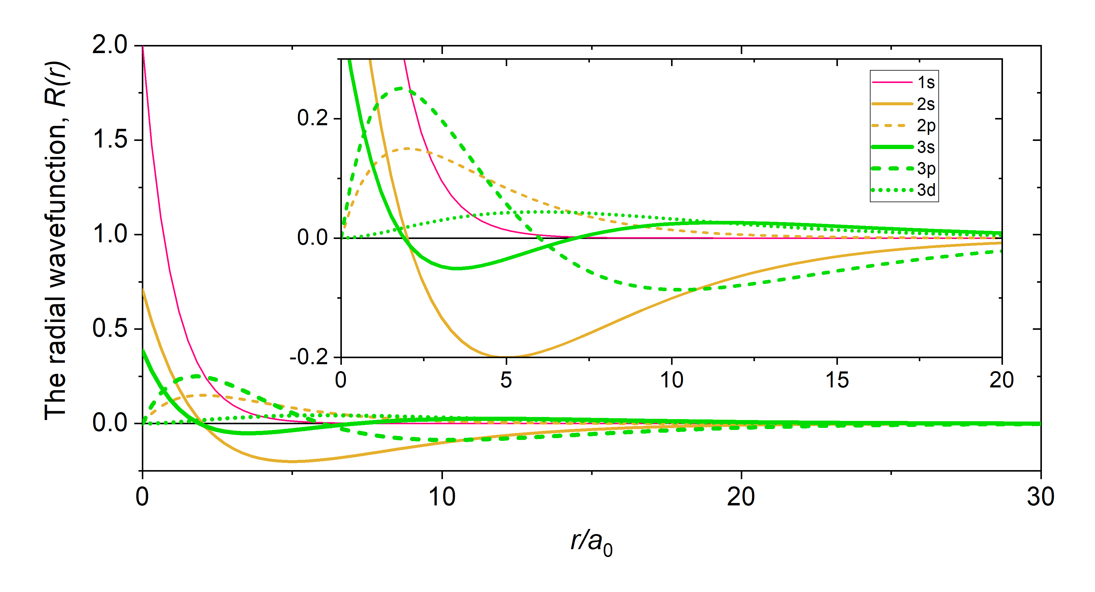
The radial part of the wavefunction, \(\textcolor{blue}{R_{n,l}(r)}\) gives the radial variation of \(\psi\). In other words, \(\textcolor{blue}{R_{n,l}(r)}\) defines how the wavefunction depends on the distance of the electron from the nucleus (the radius). The principle quantum number \(n\) is derived from the radial part of the wavefunction, and determines the size (radial extent) of an orbital. The \(\textcolor{blue}{R_{n,l}(r)}\) parts of the wavefunction for a hydrogenic atom are plotted in Figure \(\PageIndex{1}\). Notice that the \(R_{n,l}(r)\) of all s-orbitals (solid lines) reaches a maximum at \(r=0\). This is unique to the s-orbitals' \(R_{n,l}(r)\). The \(R_{n,l}(r)\) of p- and d-orbitals orbitals approaches zero as r approaches zero. This has important consequences for how closely an electron in these orbitals can approach the nucleus.
Radial probability function, \(\textcolor{black}{4 \pi r^2}\textcolor{blue}{(R_{n,l}(r))^2}\)
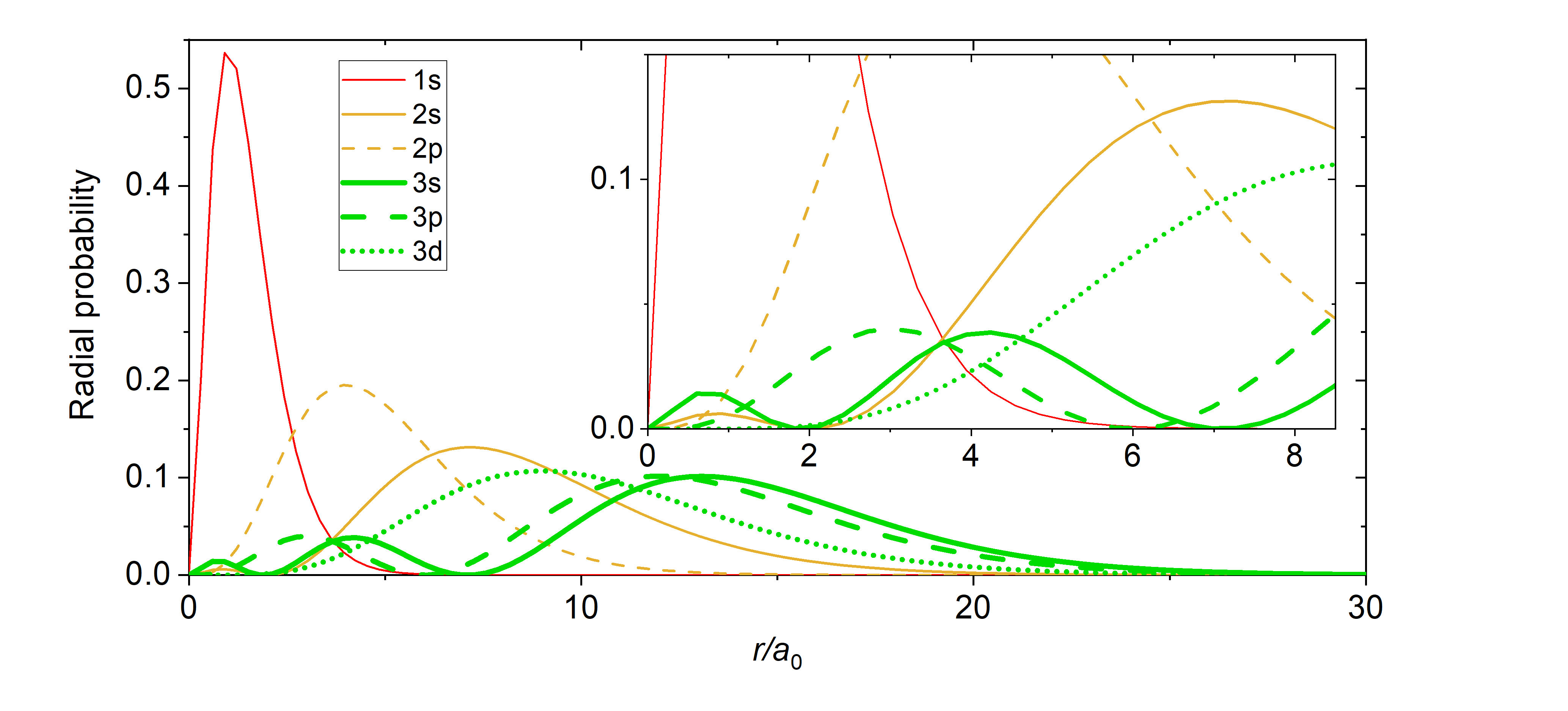
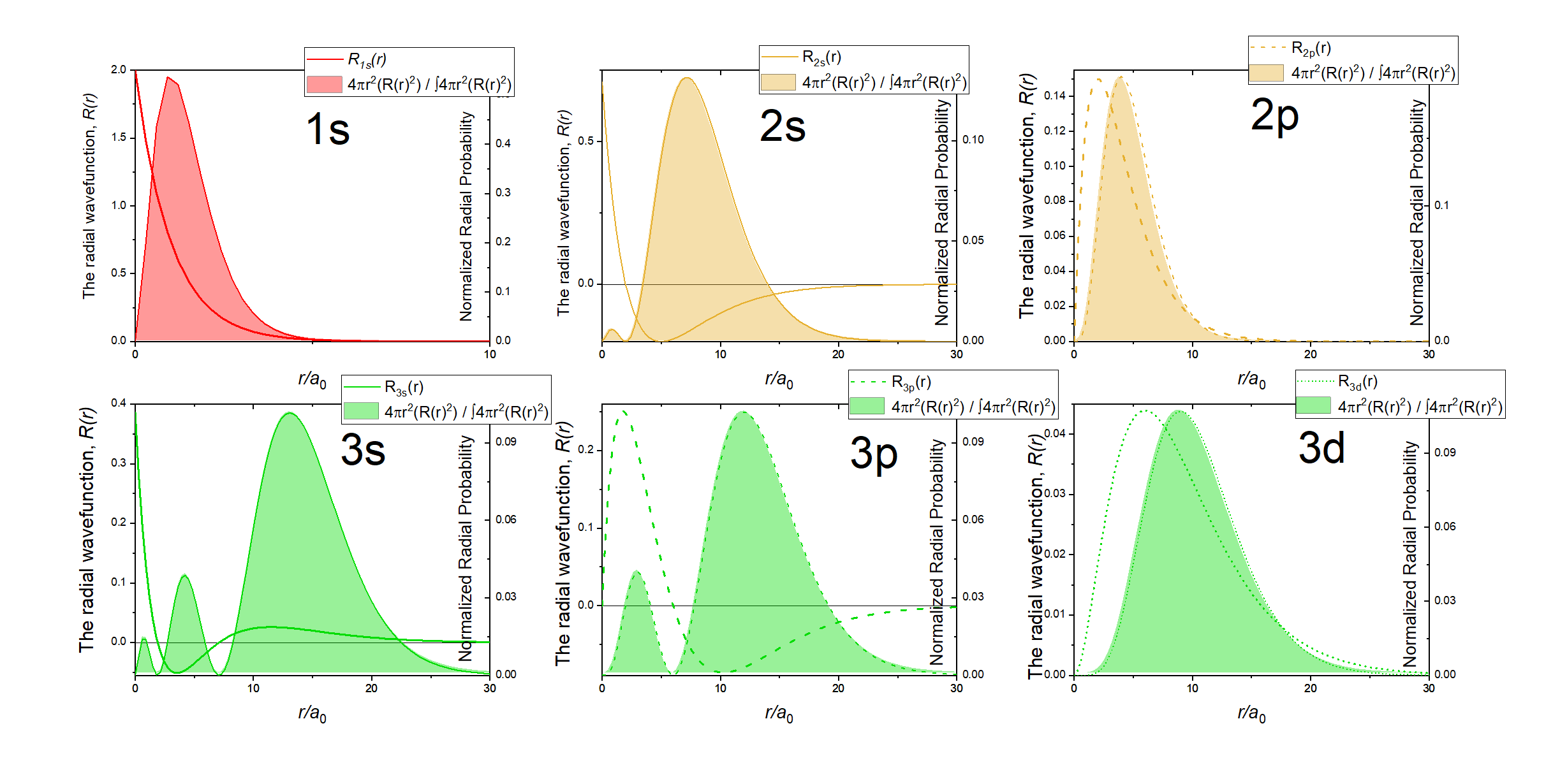
The square of the wavefunction is proportional to the probability of finding a particle (electron) at some point in space. The square of the radial part of the wavefuction is called the radial distribution function \(4 \pi r^2\textcolor{blue}{(R_{n,l}(r))^2}\), and it describes the probability of locating the electron at some distance \(r\) away from the nucleus. When we normalize the probability functions by dividing the function by its integral over all space, we get the plots shown in Figure \(\PageIndex{2}\). The normalized probability functions are compared to the original radial part of the wavefunctions in Figure \(\PageIndex{3}\). The most probable distance for finding an electron is shown by the maximum value of the function. For an electron in the 1s orbital of H, the most probable distance from the nucleus occurs at \(r=1a_0\). This is the Bohr Radius, and it has a value of (\(a_0 = 52.9 pm = 0.529 Å\)). It is convenient to plot the functions of the hydrogen atomic orbitals relative to the size of its smallest orbital, the 1s orbital; this is the reason we plot \(R_{n,l}(r)\) and \(4 \pi r^2(R_{n,l}(r))^2\) relative to \(\frac{r}{a_0}\).
Radial nodes
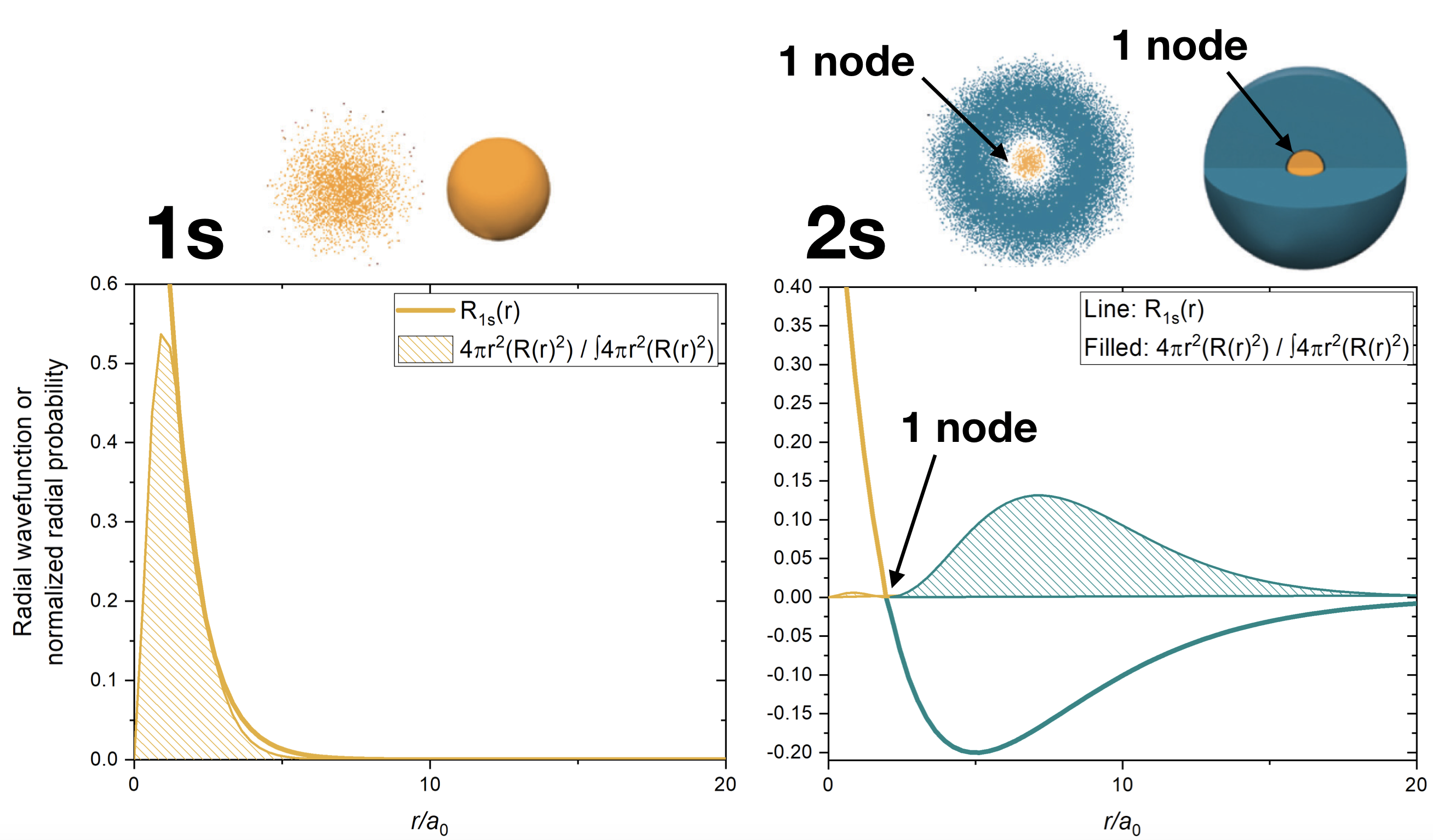
In the case of the 3-dimensional wavefunction, there are two different types of nodes: radial nodes and angular nodes. Radial nodes occur where the radial part of the wavefunction is zero (\(R(x)=0\)). These are easy to see by plotting the radial part of the wavefunction and finding where the radial part of the wavefunction (and the radial probability function) is zero as seen in Figures \(\PageIndex{2}\) and \(\PageIndex{3}\). These nodes are spherical in shape and depend on the energy level and subshell (the values of \(n\) and \(l\)). The number of radial nodes is \(n-l-1\). An example of a radial node is the single node that occurs in the \(2s\) orbital (\(2-0-1=1\) node). In contrast, the 1s orbital has zero radial nodes (\(1-0-1=0\) nodes). Where there is a node, there is zero probability of finding an electron.
Boundary surfaces
A true node occurs where the probability of finding an electron is zero. Nodes occur where \(\psi=\psi^2=0\). Far from the nucleus, the probability of finding the electron rapidly approaches zero, but is never exactly zero. What this means is that it is rather improbable to find the electron at far distances from the nucleus, but its not impossible. The rapid fall of probability creates a boundary surface rather than a node. The boundary surface represents the area around the nucleus where the electron exists most of the time.
Exercise \(\PageIndex{1}\)
How many radial nodes are in the s, p, d, and f orbitals in the first four shells? \(n=1,2,3,4\)?
- Answer
-
You can approach this answer by using the mathematical relationship between the number of radial nodes and the values of \(n\) and \(l\): number of radial nodes is \(n-1-l\). You could also notice the pattern that the first orbital of any type (1s, 2p, 3d...) has zero radial nodes, the second orbital of a type (2s, 3p, 4d...) has one radial node, the third orbital of a type has two radial nodes (3s, 4p, 5d...)...etc.
A full list of all of the orbitals in the first four shells and their number of radial nodes is below. Its a good idea to prove to yourself that the numbers given below are consistent with the plots of the orbitals wavefunctions for those orbitals in the first three shells:
s-orbitals:
1s: \(n-1-l = 1-1-0 = 0\), zero radial nodes
2s: \(n-1-l = 2-1-0 = 1\), one radial node
3s: \(n-1-l = 3-1-0 = 2\), two radial nodes
4s: \(n-1-l = 4-1-0 = 3\), three radial nodes
p-orbitals
2p: \(n-1-l = 2-1-1 = 0\), zero radial nodes
3p: \(n-1-l = 3-1-1 = 1\), one radial node
4p: \(n-1-l = 4-1-1 = 2\), two radial nodes
d-orbitals
3d: \(n-1-l = 3-1-2 = 0\), zero radial nodes
4d: \(n-1-l = 4-1-2 = 1\), one radial nodes
f-orbital
4f: \(n-1-l = 4-1-3 = 0\), zero radial nodes
Exercise \(\PageIndex{2}\)
Draw a rough plot of the following:
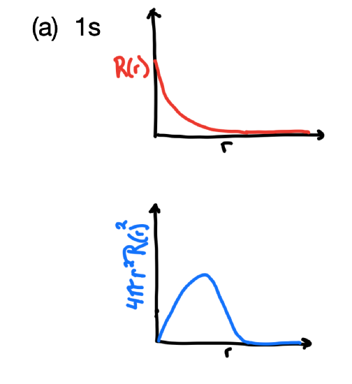
- The radial wavefunction, \(R_{n,l}(r)\) and the probability density function, \(4 \pi r^2(R_{n,l}(r))^2\), for the 1s orbital.
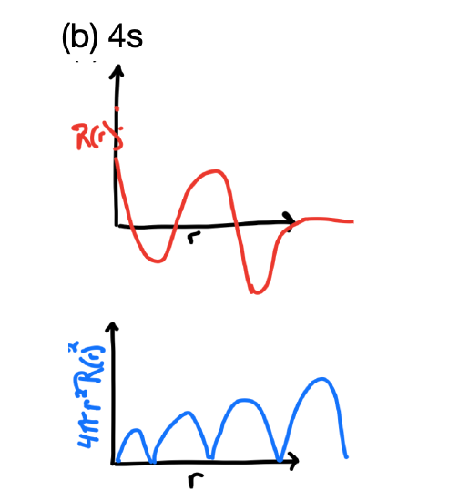
- The radial wavefunction, \(R_{n,l}(r)\) and the probability density function, \(4 \pi r^2(R_{n,l}(r))^2\), for the 4s orbital.
- Answer, 1s
-
The 1s orbital's \(R_{n,l}(r)\) reaches a maximum near the origin and approaches zero far from the nucleus. The \(4 \pi r^2(R_{n,l}(r))^2\) approaches zero at the origin, has a maximum intensity at the Bohr radius, and approaches zero far from the nucleus (its boundary surface).
 .
.
- Answer, 4s
-
Like all s orbitals, the 4s orbital's \(R_{n,l}(r)\) reaches a maximum near X=0, but it would be less intense than the function of the 1s, 2s, and 3s orbitals. It should have three radial nodes and so its wavefunction would change sign three times. This would give four regions of electron density in the probability function while the function would approach zero (boundary surface) far from the nucleus.
Angular contribution, \(\textcolor{red}{Y_{l,m_l}(\theta,\phi)}\), and angular probability function, \(\textcolor{red}{(Y_{l,m_l}(\theta,\phi))^2}\)
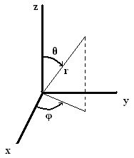 The angular contribution to the wavefunction, \(\textcolor{red}{Y_{l,m_l}(\theta,\phi)}\), describes the wavefunction's shape, or the angle with respect to a coordinate system. To describe the direction in space, we use spherical coordinates that tell us distance and orientation in 3-dimensional space. There are three spherical coordinates: \(r, \phi,\) and \(\theta\). \(r\) is the radius, or the actual distance from the origin. \(\phi\) and \(\theta\) are angles. \(\phi\) is measured from the positive x axis in the xy plane and may be between 0 and \(2\pi\). \(\theta\) is measured from the positive z axis towards the xy plane and may be between 0 and \(\pi\). \(\textcolor{red}{Y_{l,m_l}(\theta,\phi)}\), is slightly more difficult to describe than the radial contribution was. This is partly because \(\textcolor{red}{Y_{l,m_l}(\theta,\phi)}\) contains imaginary numbers, which have no real, physical meaning. However, the angular part of the wavefunction becomes more "real" when you square it to get angular probability density, a more tangible concept described as the shapes of orbitals.
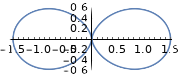
The values of \(\theta\), \(\phi\), and \(y(\theta,\phi)\) for orbitals in the hydrogen atom are listed in Table \(\PageIndex{2}\), but \(Y_{l,m_l}(\theta,\phi)\) is only a mathematical function and has not real physical meaning. The square of the radial wavefunction, \(Y_{l,m_l}(\theta,\phi)^2\) gives the probability of finding the electron at a point in space on a ray described by \((\phi, \theta)\). Thus \(Y_{l,m_l}(\theta,\phi)^2\) describes the shape of the orbital.
| subshell | \(m_l\) (orbital) | \(\theta\) | \(\phi\) | Plots of \(\theta^2\) | orbital shapes |
|---|---|---|---|---|---|
| \(l=0\), s |
\(m_l=0\) |
\(\frac{1}{\sqrt{2}}\) | \(\frac{1}{\sqrt{2 \pi}}\) |  |
|
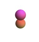
| \(l=1\), p | \(m_l=0\) | \(\frac{\sqrt{6}}{2} \cos \theta\) | \(\frac{1}{\sqrt{2 \pi}}\) |
|
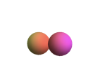 |
| \(l=1\), p | \(m_l=+1\) | \(\frac{\sqrt{3}}{2} \sin \theta\) | \(\frac{1}{\sqrt{2 \pi}} e^{i \phi}\) |  |
 |
| \(l=1\), p | \(m_l=-1\) | \(\frac{\sqrt{3}}{2} \sin \theta\) | \(\frac{1}{\sqrt{2 \pi}} e^{-i \phi}\) | 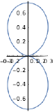 |
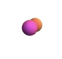 |
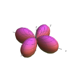
| \(l=2\), d | 0 | \(\frac{\sqrt{10}}{4}\left(3 \cos ^{2} \theta-1\right)\) | \(\frac{1}{\sqrt{2 \pi}}\) | 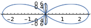 |
 |
| \(l=2\), d | \(m_l=+1\) | \(\frac{\sqrt{15}}{2} \sin \theta \cos \theta\) | \(\frac{1}{\sqrt{2 \pi}} e^{i \phi}\) |
|
 |
| \(l=2\), d | \(m_l=-1\) | \(\frac{\sqrt{15}}{2} \sin \theta \cos \theta\) | \(\frac{1}{\sqrt{2 \pi}} e^{-i \phi}\) | 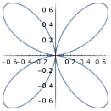 |
 |
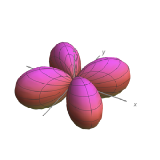
| \(l=2\), d | \(m_l=+2\) | \(\frac{\sqrt{15}}{4} \sin ^{2} \theta\) | \(\frac{1}{\sqrt{2 \pi}} e^{i 2 \phi}\) | 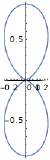 |
 |
| \(l=2\), d | \(m_l=-2\) | \(\frac{\sqrt{15}}{4} \sin ^{2} \theta\) | \(\frac{1}{\sqrt{2 \pi}} e^{-i 2 \phi}\) | |
 |
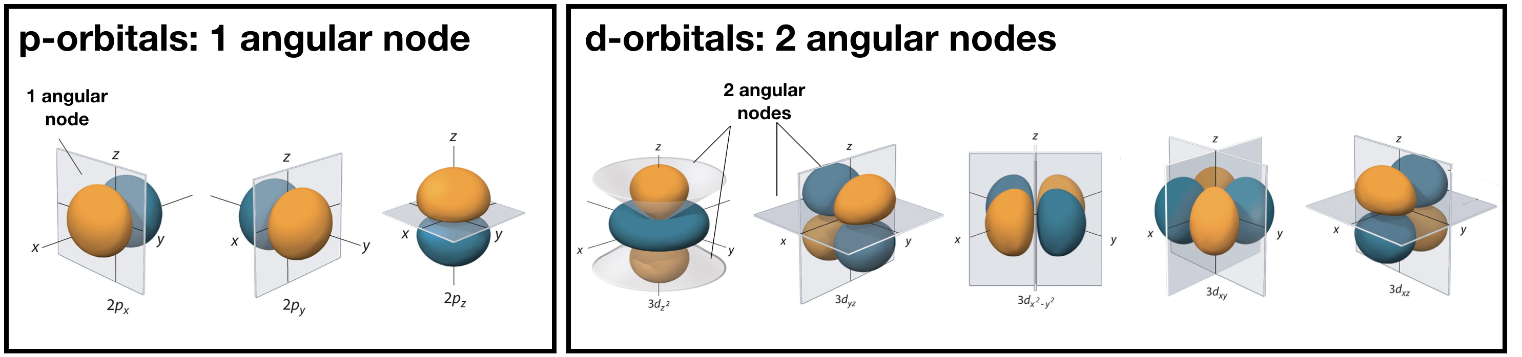
Angular nodes
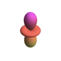
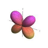
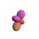
Angular nodes exist where \(\textcolor{red}{(Y_{l,m_l}(\theta,\phi))^2}=0\). These nodes are planar in shape, and they depend on the value of \(l\). The number of angular nodes in any orbital is equal to \(l\). This means that s-orbitals (\(l=0\)) have zero angular nodes, p-orbitals (\(l=1\)) have one angular node, d-orbitals (\(l=2\)) have two angular nodes, and so on. Planar nodes can be flat planes (like the nodes in all p orbitals) or they can have a conical shape, like the two angular nodes in the \(d_{Z^2}\) orbital. Angular nodes in some p and d orbitals are shown in Figure \(\PageIndex{5}\).
Atomic Orbitals
Atomic orbitals result from a combination of both the radial and angular contributions of the wavefunction. Atomic orbitals can have both angular nodes and radial nodes, depending on the values of \(n\) and \(l\).
The chart below compares the radial variation, angular variation, and their combinations (orbitals).
| Orbital | Radial Probability | Radial Nodes | Angular Probability | Angular Nodes |
Combination (Orbital) |
Total Nodes |
|---|---|---|---|---|---|---|
| 1s | 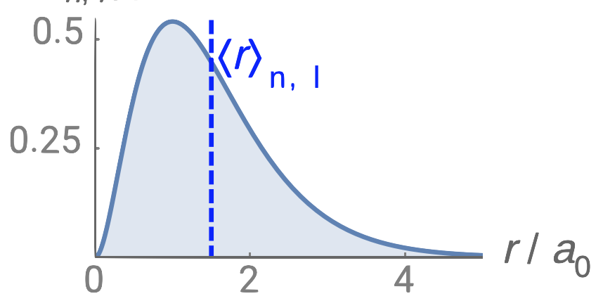 |
0 |
|
0 |  |
0 |
| 2s | 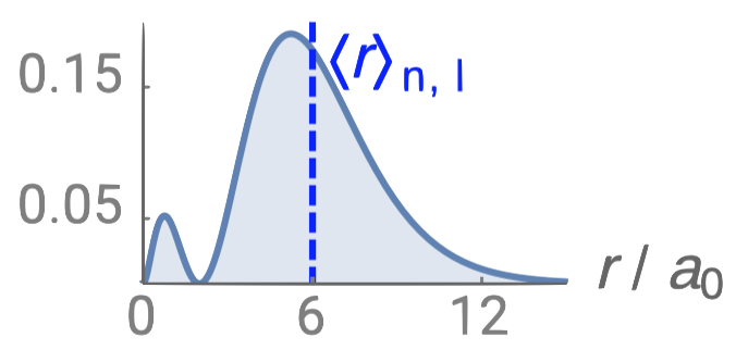 |
1 | |
0 | 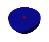 |
1 |
| 2p | 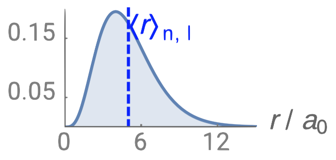 |
0 |
|
1 | 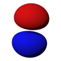 |
1 |
| 3s |  |
2 | |
0 | 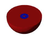 |
2 |
| 3p | 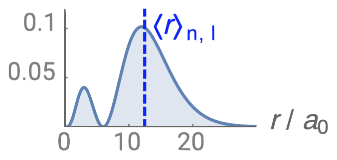 |
1 | |
1 |  |
2 |
| 3d | 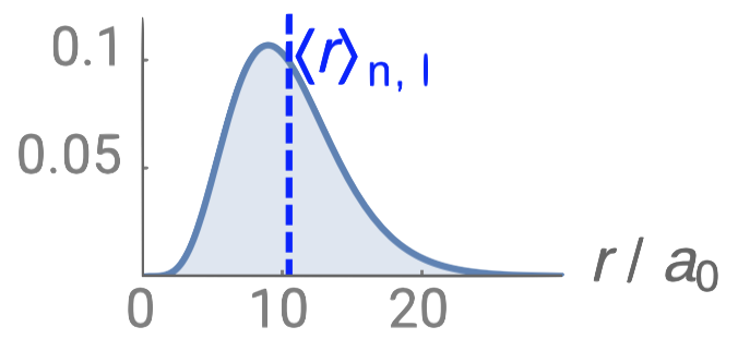 |
0 |
|
2 |  |
2 |