5.2: Introduction to Gas Chromatography Instrumentation

GC Instrumentation

In gas chromatography (GC) we inject the sample, which may be a gas or a liquid, into a gaseous mobile phase (often called the carrier gas). The mobile phase carries the sample through a stationary phase (the column) that separates the sample’s components based on their ability to partition between the mobile phase and the stationary phase. This is similar to liquid chromatography (see the HPLC module), except that the mobile phase is gas in this case. 

The instrument is called a gas chromatogram. Figure 5.2.1 shows an example of a typical gas chromatograph, which consists of several key components:

• the mobile phase; a supply of compressed gas
• a heated injector, which rapidly volatilizes the components in a liquid sample
• an oven whose temperature we can control during the separation
• a column, which is placed within the oven
• a detector to monitor the eluent as it comes off the column.

Each component will be described in detail below.

Figure 5.2.1 . Example of a typical gas chromatograph with insets showing the heated injection ports—note the symbol indicating that it is hot—and the oven that houses the column. This particular instrument is equipped with an autosampler for injecting samples, a capillary column, and a mass spectrometer (MS) as the detector. Note that the carrier gas is supplied by a tank of compressed gas.

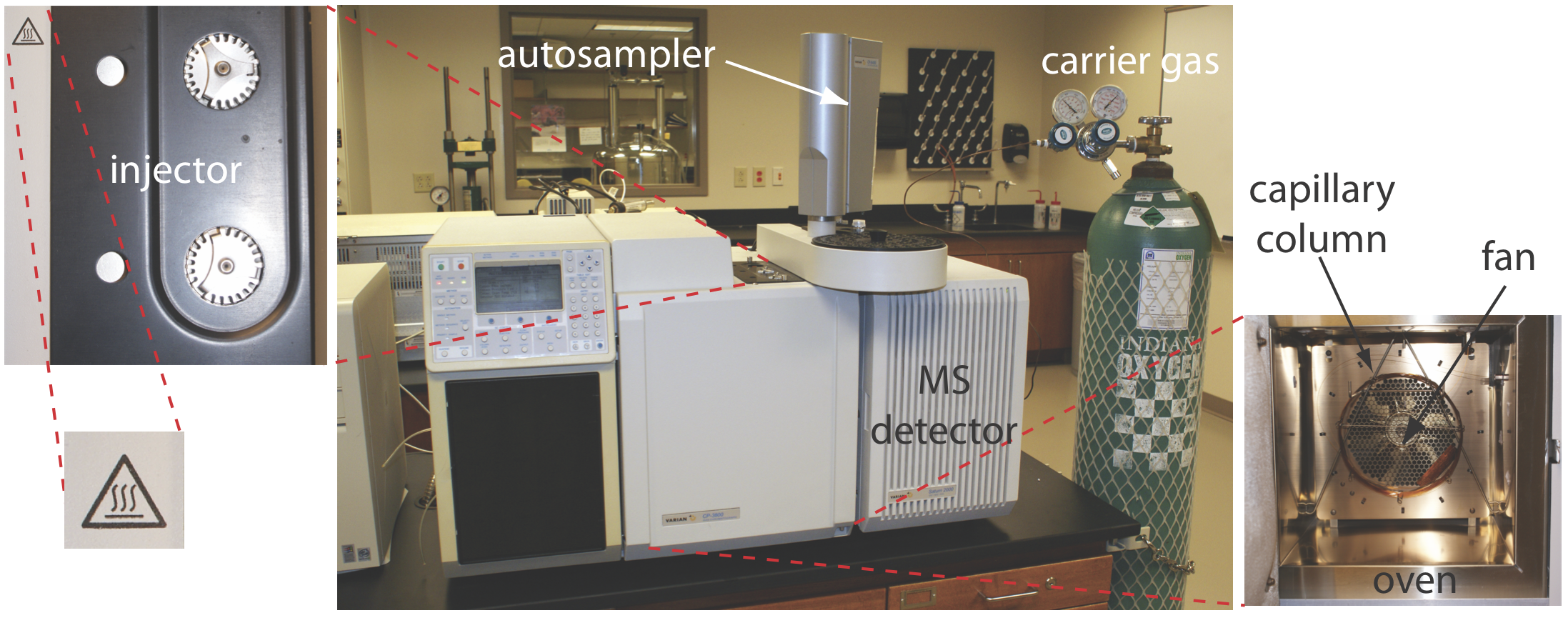
The Mobile Phase (Carrier Gas)

The mobile phase is an inert gas that does not react with the sample or the stationary phase; the most common mobile phases for gas chromatography are He, Ar, and N₂. The choice of carrier gas often is determined by the needs of instrument’s detector. The flow rates depend on the type of column; it is usually 25–150 mL/min for a packed column and 1–25 mL/min for a capliary column.

The Stationary Phase (Column)

There are two broad classes of chromatographic columns: packed columns and capillary columns. In general, a packed column can handle larger samples and a capillary column can separate more complex mixtures. Only the caplilary column is described here.

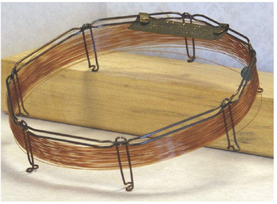
A capillary, or open tubular column is constructed from fused silica and is coated with a protective polymer coating. Columns range from 15–100 m in length with an internal diameter of approximately 150–300 μm. Figure 5.2.3 shows an example of a typical capillary column.

Figure 5.2.3 . Typical example of a capillary column for gas chromatography. This column is 30 m long with an internal diameter of 247 μm. The interior surface of the capillary has a 0.25 μm coating of the liquid phase.

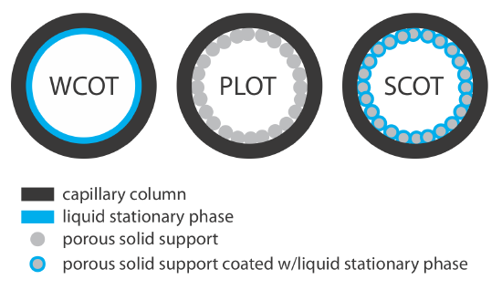
Capillary columns are of three principal types. In a wall-coated open tubular column (WCOT) a thin layer of stationary phase, typically 0.25 nm thick, is coated on the capillary’s inner wall. In a porous-layer open tubular column (PLOT), a porous solid support—alumina, silica gel, and molecular sieves are typical examples—is attached to the capillary’s inner wall. A support-coated open tubular column (SCOT) is a PLOT column that includes a liquid stationary phase. Figure 5.2.4 shows the differences between these types of capillary columns.

Figure 5.2.4 . Cross sections through the three types of capillary columns.

A capillary column provides a significant improvement in separation efficiency because it has more theoretical plates per meter and is longer than a packed column. For example, the capillary column in Figure 5.2.3 has almost 4300 plates/m, or a total of 129 000 theoretical plates. If we assume a V_max/V_min ≈ 50, then it has a peak capacity of approximately 350. On the other hand, a packed column can handle a larger sample. Because of its smaller diameter, a capillary column requires a smaller sample, typically less than 10^–2 μL.

Choice of stationary phase

Elution order in gas–liquid chromatography depends on two factors: the boiling point of the solutes, and the interaction between the solutes and the stationary phase. If a mixture’s components have significantly different boiling points, then the choice of stationary phase is less critical. If two solutes have similar boiling points, then a separation is possible only if the stationary phase selectively interacts with one of the solutes. As a general rule, nonpolar solutes are separated more easily when using a nonpolar stationary phase, and polar solutes are easier to separate when using a polar stationary phase.

There are several important criteria for choosing a stationary phase: it must not react with the solutes, it must be thermally stable, it must have a low volatility, and it must have a polarity that is appropriate for the sample’s components.

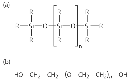
Many stationary phases have the general structure shown in Figure 5.2.5 a. A stationary phase of polydimethyl siloxane, in which all the –R groups are methyl groups, –CH₃, is nonpolar and often makes a good first choice for a new separation. The order of elution when using polydimethyl siloxane usually follows the boiling points of the solutes, with lower boiling solutes eluting first. Replacing some of the methyl groups with other substituents increases the stationary phase’s polarity and provides greater selectivity. For example, replacing 50% of the –CH₃ groups with phenyl groups, –C₆H₅, produces a slightly polar stationary phase. Increasing polarity is provided by substituting trifluoropropyl, –C₃H₆CF, and cyanopropyl, –C₃H₆CN, functional groups, or by using a stationary phase of polyethylene glycol (Figure 5.2.5 b).

Figure 5.2.5 . General structures of common stationary phases: (a) substituted polysiloxane; (b) polyethylene glycol.

An important problem with all liquid stationary phases is their tendency to elute, or bleed from the column when it is heated. The temperature limits in Table 5.2.1 minimize this loss of stationary phase. Capillary columns with bonded or cross-linked stationary phases provide superior stability. A bonded stationary phase is attached chemically to the capillary’s silica surface. Cross-linking, which is done after the stationary phase is in the capillary column, links together separate polymer chains to provide greater stability.

Another important consideration is the thickness of the stationary phase. From equation 12.3.7 we know that separation efficiency improves with thinner film of stationary phase. The most common thickness is 0.25 μm, although a thicker films is useful for highly volatile solutes, such as gases, because it has a greater capacity for retaining such solutes. Thinner films are used when separating low volatility solutes, such as steroids.

A few stationary phases take advantage of chemical selectivity. The most notable are stationary phases that contain chiral functional groups, which are used to separate enantiomers [Hinshaw, J. V. LC .GC 1993, 11, 644–648].

Sample Introduction

Three factors determine how we introduce a sample to the gas chromatograph. First, all of the sample’s constituents must be volatile. Second, the analytes must be present at an appropriate concentration. Finally, the physical process of injecting the sample must not degrade the separation. Each of these needs is considered in this section.

Preparing a Volatile Sample

Not every sample can be injected directly into a gas chromatograph. To move through the column, the sample’s constituents must be sufficiently volatile. A solute of low volatility, for example, may be retained by the column and continue to elute during the analysis of subsequent samples. A nonvolatile solute will condense at the top of the column, degrading the column’s performance.

We can separate a sample’s volatile analytes from its nonvolatile components using any of the extraction techniques described in Chapter 7. A liquid–liquid extraction of analytes from an aqueous matrix into methylene chloride or another organic solvent is a common choice. Solid-phase extractions also are used to remove a sample’s nonvolatile components.

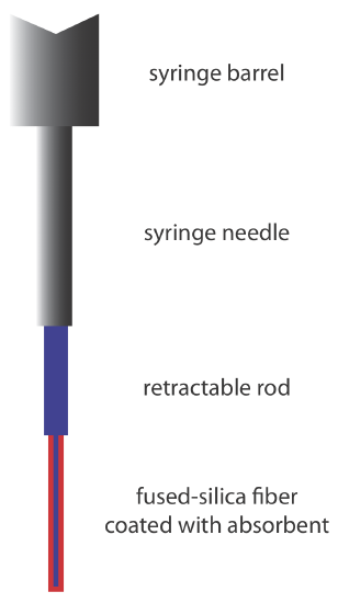
An attractive approach to isolating analytes is a solid-phase microextraction (SPME). In one approach, which is illustrated in Figure 5.2.6 , a fused-silica fiber is placed inside a syringe needle. The fiber, which is coated with a thin film of an adsorbent material, such as polydimethyl siloxane, is lowered into the sample by depressing a plunger and is exposed to the sample for a predetermined time. After withdrawing the fiber into the needle, it is transferred to the gas chromatograph for analysis.

Figure 5.2.6 . Schematic diagram of a solid-phase microextraction device. The absorbent is shown in red.

Two additional methods for isolating volatile analytes are a purge-and-trap and headspace sampling. In a purge-and-trap, we bubble an inert gas, such as He or N₂, through the sample, releasing—or purging—the volatile compounds. These compounds are carried by the purge gas through a trap that contains an absorbent material, such as Tenax, where they are retained. Heating the trap and back-flushing with carrier gas transfers the volatile compounds to the gas chromatograph. In headspace sampling we place the sample in a closed vial with an overlying air space. After allowing time for the volatile analytes to equilibrate between the sample and the overlying air, we use a syringe to extract a portion of the vapor phase and inject it into the gas chromatograph. Alternatively, we can sample the headspace with an SPME.

Thermal desorption is a useful method for releasing volatile analytes from solids. We place a portion of the solid in a glass-lined, stainless steel tube. After purging with carrier gas to remove any O₂ that might be present, we heat the sample. Volatile analytes are swept from the tube by an inert gas and carried to the GC. Because volatilization is not a rapid process, the volatile analytes often are concentrated at the top of the column by cooling the column inlet below room temperature, a process known as cryogenic focusing. Once volatilization is complete, the column inlet is heated rapidly, releasing the analytes to travel through the column.

The reason for removing O₂ is to prevent the sample from undergoing an oxidation reaction when it is heated.

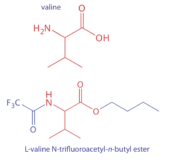
To analyze a nonvolatile analyte we must convert it to a volatile form. For example, amino acids are not sufficiently volatile to analyze directly by gas chromatography. Reacting an amino acid, such as valine, with 1-butanol and acetyl chloride produces an esterified amino acid. Subsequent treatment with trifluoroacetic acid gives the amino acid’s volatile N-trifluoroacetyl-n-butyl ester derivative.

Adjusting the Analyte's Concentration

In an analyte’s concentration is too small to give an adequate signal, then we must concentrate the analyte before we inject the sample into the gas chromatograph. A side benefit of many extraction methods is that they often concentrate the analytes. Volatile organic materials isolated from an aqueous sample by a purge-and-trap, for example, are concentrated by as much as \(1000 \times\).

If an analyte is too concentrated, it is easy to overload the column, resulting in peak fronting (see Figure 12.2.7) and a poor separation. In addition, the analyte’s concentration may exceed the detector’s linear response. Injecting less sample or diluting the sample with a volatile solvent, such as methylene chloride, are two possible solutions to this problem.

Injecting the Sample

In Chapter 12.3 of Harvey's Analytical Text, he describes several explanations for why a solute’s band increases in width as it passes through the column, a process we called band broadening. We also introduce an additional source of band broadening if we fail to inject the sample into the minimum possible volume of mobile phase. There are two principal sources of this precolumn band broadening: injecting the sample into a moving stream of mobile phase and injecting a liquid sample instead of a gaseous sample. The design of a gas chromatograph’s injector helps minimize these problems.

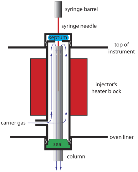
An example of a simple injection port for a packed column is shown in Figure 5.2.7 . The top of the column fits within a heated injector block, with carrier gas entering from the bottom. The sample is injected through a rubber septum using a microliter syringe, such as the one shown in in Figure 5.2.8 . Injecting the sample directly into the column minimizes band broadening because it mixes the sample with the smallest possible amount of carrier gas. The injector block is heated to a temperature at least 50^oC above the boiling point of the least volatile solute, which ensures a rapid vaporization of the sample’s components.

Figure 5.2.7 . Schematic diagram of a heated GC injector port for use with packed columns. The needle pierces a rubber septum and enters into the top of the column, which is located within a heater block.

Figure 5.2.8 . Example of a syringe for injecting samples into a gas chromatograph. This syringe has a maximum capacity of 10 μL with graduations every 0.1 μL.

Because a capillary column’s volume is significantly smaller than that for a packed column, it requires a different style of injector to avoid overloading the column with sample. Figure 5.2.9 shows a schematic diagram of a typical split/splitless injector for use with a capillary column.

Figure 5.2.9 . Schematic diagram of a split/splitless injection port for use with capillary columns. The needle pierces a rubber septum and enters into a glass liner, which is located within a heater block. In a split injection the split vent is open; the split vent is closed for a splitless injection.

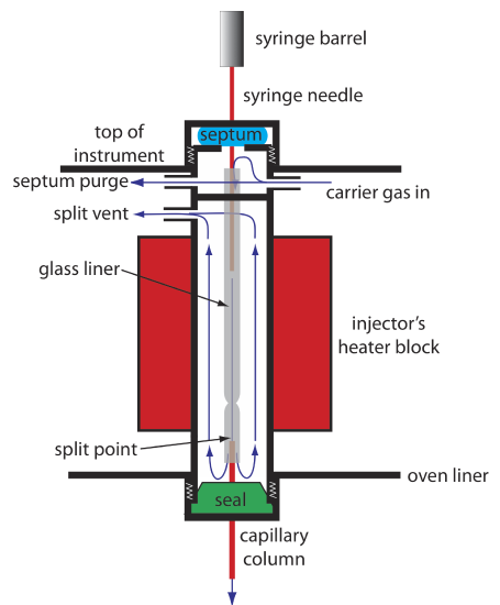
In a split injection we inject the sample through a rubber septum using a microliter syringe. Instead of injecting the sample directly into the column, it is injected into a glass liner where it mixes with the carrier gas. At the split point, a small fraction of the carrier gas and sample enters the capillary column with the remainder exiting through the split vent. By controlling the flow rate of the carrier gas as it enters the injector, and its flow rate through the septum purge and the split vent, we can control the fraction of sample that enters the capillary column, typically 0.1–10%.

For example, if the carrier gas flow rate is 50 mL/min, and the flow rates for the septum purge and the split vent are 2 mL/min and 47 mL/min, respectively, then the flow rate through the column is 1 mL/min (= 50 – 2 – 47). The ratio of sample entering the column is 1/50, or 2%.

In a splitless injection, which is useful for trace analysis, we close the split vent and allow all the carrier gas that passes through the glass liner to enter the column—this allows virtually all the sample to enters the column. Because the flow rate through the injector is low, significant precolumn band broadening is a problem. Holding the column’s temperature approximately 20–25^oC below the solvent’s boiling point allows the solvent to condense at the entry to the capillary column, forming a barrier that traps the solutes. After allowing the solutes to concentrate, the column’s temperature is increased and the separation begins.

For samples that decompose easily, an on-column injection may be necessary. In this method the sample is injected directly into the column without heating. The column temperature is then increased, volatilizing the sample with as low a temperature as is practical.

Oven with Temperature Control

In gas chromatography a sample is injected into a column containing a stationary phase composed either of a packed, liquid-coated solid support material (a “packed” column) or a high molecular weight, thermally stable polymer film coating the column inner wall (a capillary column). The sample is carried through the column by an inert "carrier gas" (the mobile phase). Because of their different affinities for the stationary phase the individual components of the sample mixture pass through the column at different rates, eluting separately from the column at characteristic retention times. In a typical GC experiment the column temperature and carrier gas flow rate both affect the quality of the separation. With regard to the column temperature, two types of GC experiments should be considered, isothermal (constant temperature) and temperature programmed.

Isothermal Gas Chromatography

In an isothermal separation we maintain the column at a constant temperature. To increase the interaction between the solutes and the stationary phase, the temperature usually is set slightly below that of the lowest-boiling solute. 

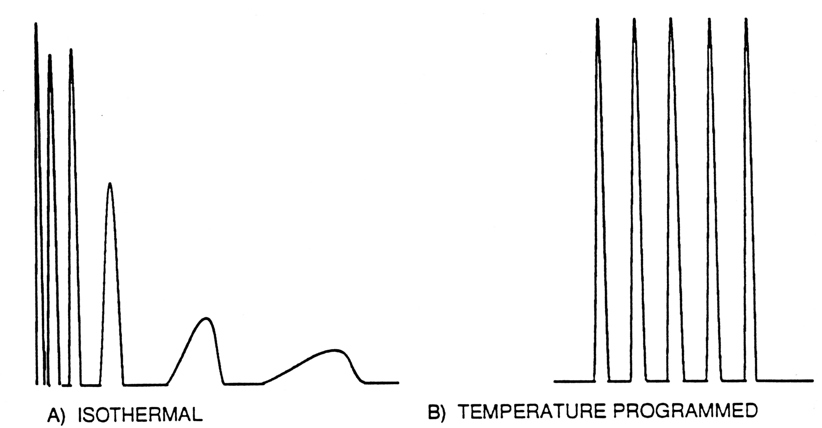
Consider, for example, the separation of members of a homologous series such as the n- alkanes. As shown in Figure \(\PageIndex{9}\), Panel A, in an isothermal experiment one expects the retention times of the solutes to vary as a function of boiling point. Indeed, the boiling points, and similarly, the heats of vaporization, ∆Hv, have been shown to increase linearly with increasing carbon number, which is related to molar volume. It has also been shown that the retention volume, \(\mathrm{V}_{\mathrm{r}}\), is related to \(-\Delta \mathrm{H}_{\mathrm{V}}\) by the equation below where R is the gas constant and T is the column temperature used in the chromatographic experiment. Based on the above equation it is evident that a linear relationship also exists between \(\ln \mathrm{V}_{\mathrm{r}}\) and 1/T, and that at constant temperature a linear relationship should exist between \(\mathrm{V}_{\mathrm{r}}\) and carbon number in the homologous series.

\[\ln \mathrm{V}_{\mathrm{r}}=\left(-\Delta \mathrm{H}_{\mathrm{V}} / \mathrm{RT}\right)+\mathrm{constant} \label{rv}\]

Figure \(\PageIndex{9}\): Example of an Isothermal Gas Chromatogram. (Copyright; author via source)

From the known relationship \(\mathrm{V}_{\mathrm{r}}=\mathrm{V}_{\mathrm{o}}+\mathrm{KV}_{\mathrm{S}}\) and \(\mathrm{k}^{\prime}=\mathrm{KV}_{\mathrm{S}} / \mathrm{V}_{\mathrm{O}}\) where Vo is the column dead volume, K is the partition coefficient for a particular volatile component, Vs is the volume of the stationary phase, and k' is the capacity factor, a net retention parameter, it can be shown that \[\mathrm{k}^{\prime}=\left(\mathrm{V}_{\mathrm{r}}-\mathrm{V}_{\mathrm{o}}\right) / \mathrm{V}_{\mathrm{o}} \label{capacity}\]

For a constant flow rate, F, Vr = trF (tr = total retention time), and Vo = toF (to = retention time of an un-retained species). Equation \ref{capacity} can be rewritten as: \[\mathrm{k}^{\prime}=\left(\mathrm{t}_{\mathrm{r}}-\mathrm{t}_{\mathrm{o}}\right) / \mathrm{t}_{\mathrm{O}}\]

Since k' is proportional to Vr, Equation \ref{rv} can then be written in the following form:

\[\ln \left[\left(\mathrm{t}_{\mathrm{r}}-\mathrm{t}_{\mathrm{o}}\right) / \mathrm{t}_{\mathrm{o}}\right]=\left(-\Delta \mathrm{H}_{\mathrm{v}} / \mathrm{RT}\right)+\text { constant }\]

Thus, a linear relationship should result from plotting the measured retention times for a homologous series verses carbon number.

The advantage of an isothermal experiment is that the theory suggests that this linear relationship will hold for the separation of a homologous series of compounds. The disadvantage is that, in practice, when a large number of samples with a wide range in physical- chemical properties are separated, peaks for compounds of low boiling points tend to be crowded together at the beginning of the chromatogram while the slow moving, high boiling components tend to appear as severely broadened peaks with impractically long retention times (Figure \(\PageIndex{9}\)). The most common way to solve this problem is to use temperature programmed gas chromatography (TPGC).

Temperature Programed Gas Chromatography (TPGC)

One difficulty with an isothermal separation is that a temperature that favors the separation of a low-boiling solute may lead to an unacceptably long retention time for a higher-boiling solute. Temperature programming provides a solution to this problem. At the beginning of the analysis we set the column’s initial temperature below that for the lowest-boiling solute. As the separation progresses, we slowly increase the temperature at either a uniform rate or in a series of steps.

When a sample is injected into a gas chromatograph, individual components of the sample mixture pass through the column at different rates, eluting separately from the column at characteristic retention times depending on their affinity for the stationary phase, the temperature of the column, and the rate of flow of carrier gas. An optimized separation involves the correct balancing of these conditions. By slowly raising the temperature of the column during the separation process, each component may be eluted at its optimum temperature for the flow rate chosen. In general the minimum and maximum temperatures should bracket the boiling points of the most and least volatile components of the sample. The rate at which heating is to take place is dependent on the number and the retention spacing of the components to be separated. Figure \(\PageIndex{9}\) shows how typical isothermal chromatogram (Figure \(\PageIndex{9}\)A) is optimized by TPGC (Figure \(\PageIndex{9}\)B). It is found experimentally that when a constant heating rate is used the mathematical formulas described above in Equations \ref{rv} - \ref{capacity} tend to hold and thus we tend to see the expected linear relationships between members of a homologous series of compounds.

Detectors for Gas Chromatography

The final part of a gas chromatograph is the detector. The ideal detector has several desirable features: a low detection limit, a linear response over a wide range of solute concentrations (which makes quantitative work easier), sensitivity for all solutes or selectivity for a specific class of solutes, and an insensitivity to a change in flow rate or temperature. This section will describe the two types of detectors that are available in the undergraduate teaching labs at Duke. If you are interested in learning what other types of detectors can be used with GC, see 12.4: Gas Chromatography by David Harvey.

Flame Ionization Detector (FID)

The combustion of an organic compound in an H₂/air flame results in a flame that contains electrons and organic cations, presumably CHO⁺. Applying a potential of approximately 300 volts across the flame creates a small current of roughly 10^–9 to 10^–12 amps. When amplified, this current provides a useful analytical signal. This is the basis of the popular flame ionization detector, a schematic diagram of which is shown in Figure 5.2.10 .

Figure 5.2.10 . Schematic diagram of a flame ionization detector. The eluent from the column mixes with H₂ and is burned in the presence of excess air. Combustion produces a flame that contains electrons and the cation CHO^+. Applying a potential between the flame’s tip and the collector gives a current that is proportional to the concentration of cations in the flame.

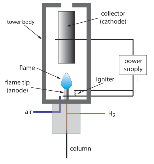
Most carbon atoms—except those in carbonyl and carboxylic groups—generate a signal, which makes the FID an almost universal detector for organic compounds. Most inorganic compounds and many gases, such as H₂O and CO₂, are not detected, which makes the FID detector a useful detector for the analysis of organic analytes in atmospheric and aqueous environmental samples. Advantages of the FID include a detection limit that is approximately two to three orders of magnitude smaller than that for a thermal conductivity detector, and a linear response over 10⁶–10⁷ orders of magnitude in the amount of analyte injected. The sample, of course, is destroyed when using a flame ionization detector.

Mass Spectrometer (MS)

A mass spectrometer is an instrument that ionizes a gaseous molecule using sufficient energy that the resulting ion breaks apart into smaller ions. Because these ions have different mass-to-charge ratios, it is possible to separate them using a magnetic field or an electrical field. The resulting mass spectrum contains both quantitative and qualitative information about the analyte. Figure 5.2.11 shows a mass spectrum for toluene.

Figure 5.2.11 . Mass spectrum for toluene highlighting the molecular ion in green (m/z=92), and two fragment ions in blue (m/z=91) and in red (m/z= 65). A mass spectrum provides both quantitative and qualitative information: the height of any peak is proportional to the amount of toluene in the mass spectrometer and the fragmentation pattern is unique to toluene.

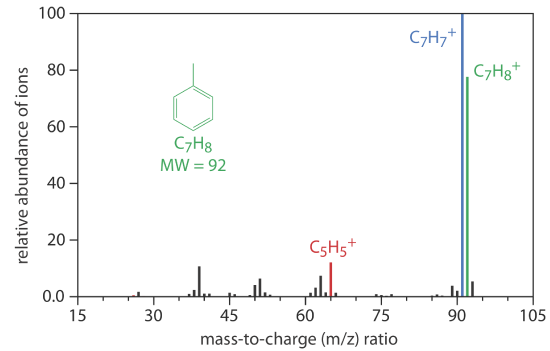
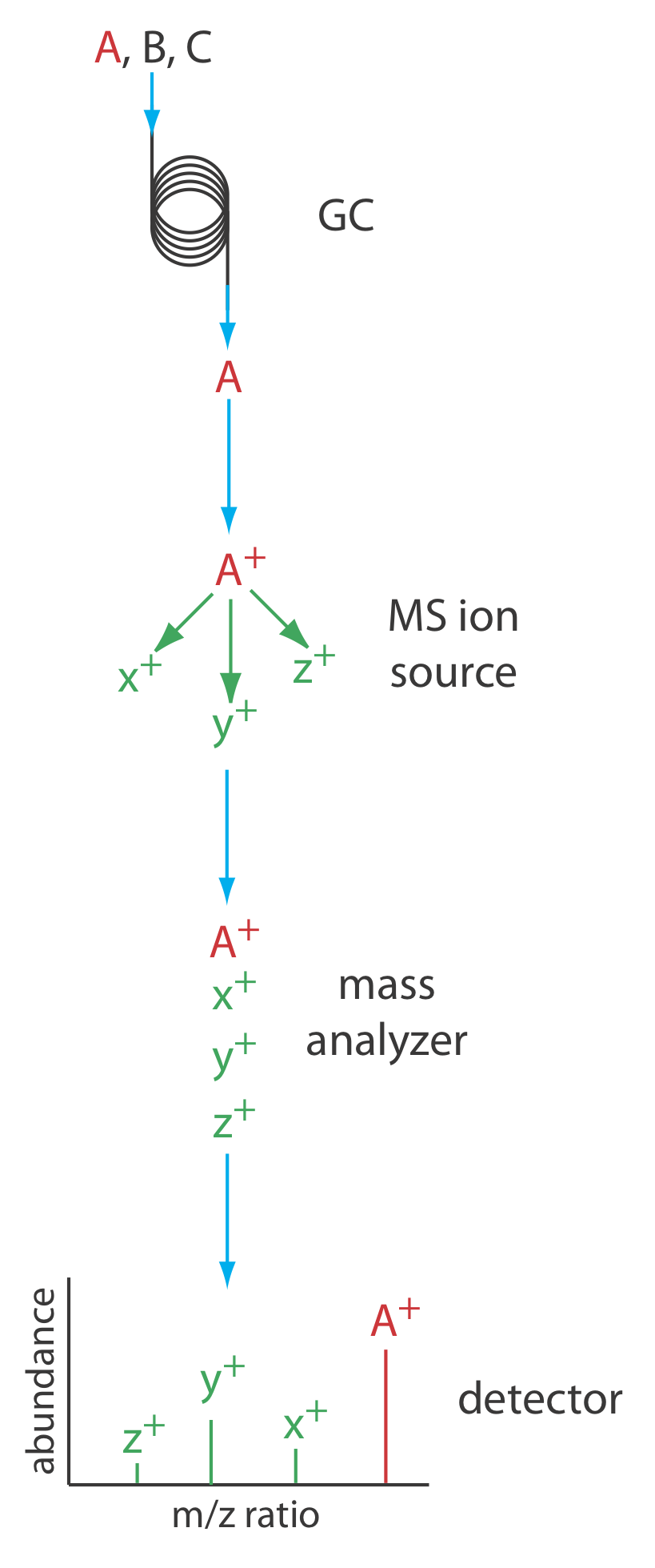
Figure 5.2.14 shows a block diagram of a typical gas chromatography-mass spectrometer (GC–MS) instrument. The effluent from the column enters the mass spectrometer’s ion source in a manner that eliminates the majority of the carrier gas. In the ionization chamber the remaining molecules—a mixture of carrier gas, solvent, and solutes—undergo ionization and fragmentation. The mass spectrometer’s mass analyzer separates the ions by their mass-to-charge ratio and a detector counts the ions and displays the mass spectrum.

Figure 5.2.14 . Block diagram of GC– MS. A three component mixture enters the GC. When component A elutes from the column, it enters the MS ion source and ionizes to form the parent ion and several fragment ions. The ions enter the mass analyzer, which separates them by their mass-to-charge ratio, providing the mass spectrum shown at the detector.

There are several options for monitoring a chromatogram when using a mass spectrometer as the detector. The most common method is to continuously scan the entire mass spectrum and report the total signal for all ions that reach the detector during each scan. This total ion scan provides universal detection for all analytes. We can achieve some degree of selectivity by monitoring one or more specific mass-to-charge ratios, a process called selective-ion monitoring. A mass spectrometer provides excellent detection limits, typically 25 fg to 100 pg, with a linear range of 10⁵ orders of magnitude. Because we continuously record the mass spectrum of the column’s eluent, we can go back and examine the mass spectrum for any time increment. This is a distinct advantage for GC–MS because we can use the mass spectrum to help identify a mixture’s components.

For more details on mass spectrometry see Introduction to Mass Spectrometry by Michael Samide and Olujide Akinbo, a resource that is part of the Analytical Sciences Digital Library.