3.3: UV/Vis Instrumentation

In this section, we examine several different instruments for U-vis absorption spectroscopy, with an emphasis on the specific instruments used in our teaching labs at Duke, and their advantages and limitations. Methods of sample introduction are also covered in this section form more information about absorption spectroscopy, or for a description of the clinical, environmental, and other applications of absorption spectroscopy, see 10.3: UV/Vis and IR Spectroscopies by David Harvey.

Instrument Designs for Molecular UV/Vis Absorption

Single-Beam Spectrophotometer.

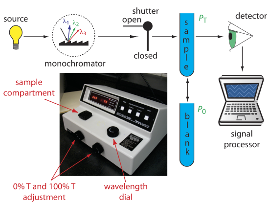
An instrument that uses a monochromator for wavelength selection is called a spectrophotometer. The simplest spectrophotometer is a single-beam instrument equipped with a fixed-wavelength monochromator (Figure 3.3.2 ). Single-beam spectrophotometers are calibrated and used in the same manner as a photometer. One example of a single-beam spectrophotometer is Thermo Scientific’s Spectronic 20D+, which is shown in the photographic insert to Figure 3.3.2 . This is similar to the Genesys Spec 20 that you used in the previous module.

The Spectronic 20D+ has a wavelength range of 340–625 nm (950 nm when using a red-sensitive detector), and a fixed effective bandwidth of 20 nm. Battery-operated, hand-held single-beam spectrophotometers are available, which are easy to transport into the field. Other single-beam spectrophotometers also are available with effective bandwidths of 2–8 nm. Fixed wavelength single-beam spectrophotometers are not practical for recording spectra because manually adjusting the wavelength and recalibrating the spectrophotometer is awkward and time-consuming. The accuracy of a single-beam spectrophotometer is limited by the stability of its source and detector over time.

Figure 3.3.2 . Schematic diagram of a fixed-wavelength, single-beam spectrophotometer. The photographic inset shows a typical instrument. The shutter remains closed until the sample or blank is placed in the sample compartment. The analyst manually selects the wavelength by adjusting the wavelength dial. Inset photo modified from: Adi (www.commons.Wikipedia.org).

Double-Beam Spectrophotometer.

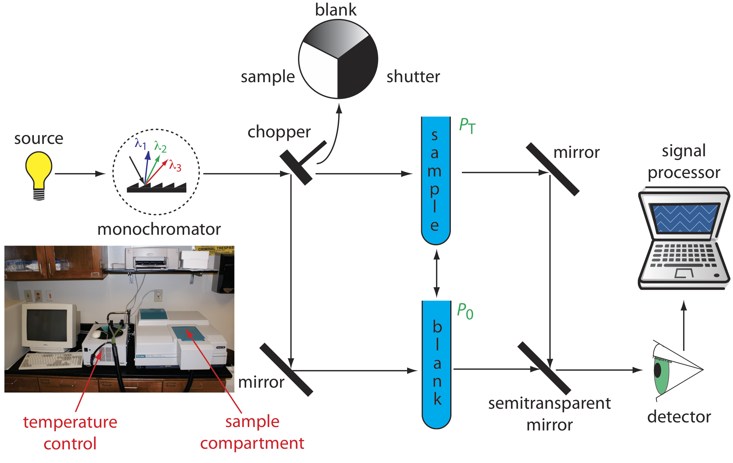
The limitations of a fixed-wavelength, single-beam spectrophotometer is minimized by using a double-beam spectrophotometer (Figure 3.3.3 ). A chopper controls the radiation’s path, alternating it between the sample, the blank, and a shutter. The signal processor uses the chopper’s speed of rotation to resolve the signal that reaches the detector into the transmission of the blank, P₀, and the sample, P_T. By including an opaque surface as a shutter, it also is possible to continuously adjust 0%T. The effective bandwidth of a double-beam spectrophotometer is controlled by adjusting the monochromator’s entrance and exit slits. Effective bandwidths of 0.2–3.0 nm are common. A scanning monochromator allows for the automated recording of spectra. Double-beam instruments are more versatile than single-beam instruments, being useful for both quantitative and qualitative analyses, but also are more expensive and not particularly portable. You will use a double-beam spectrometer in this UV-vis module of this course, and the instrument you will use is the same as that pictured in Figure 3.3.3 ; it is an Agilent Cary UV-vis double beam spectrometer. 

Figure 3.3.3 . Schematic diagram of a scanning, double-beam spectrophotometer. A chopper directs the source’s radiation, using a transparent window to pass radiation to the sample and a mirror to reflect radiation to the blank. The chopper’s opaque surface serves as a shutter, which allows for a constant adjustment of the spectrophotometer’s 0%T. The photographic insert shows a typical instrument. The module in the middle of the photo is a temperature control unit that makes it possible to heat or cool the sample to a constant temperature.

Diode Array Spectrometer

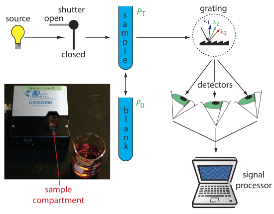
An instrument with a single detector can monitor only one wavelength at a time. If we replace a single photomultiplier with an array of photodiodes, we can use the resulting detector to record a full spectrum in as little as 0.1 s. In a diode array spectrometer the source radiation passes through the sample and is dispersed by a grating (Figure 3.3.4 ). The photodiode array detector is situated at the grating’s focal plane, with each diode recording the radiant power over a narrow range of wavelengths. Because we replace a full monochromator with just a grating, a diode array spectrometer is small and compact. This is the kind of spectrometer that is integrated into the Duke teach labs' HPLC system as an in-line detector. It is also the type of detector that is used in our Agilent Cary 60 spectrometer.

Figure 3.3.4 . Schematic diagram of a diode array spectrophotometer. The photographic insert shows a typical instrument. Note that the 50-mL beaker provides a sense of scale. Because the spectrometer is small and compact, it is easy to transport into the field.

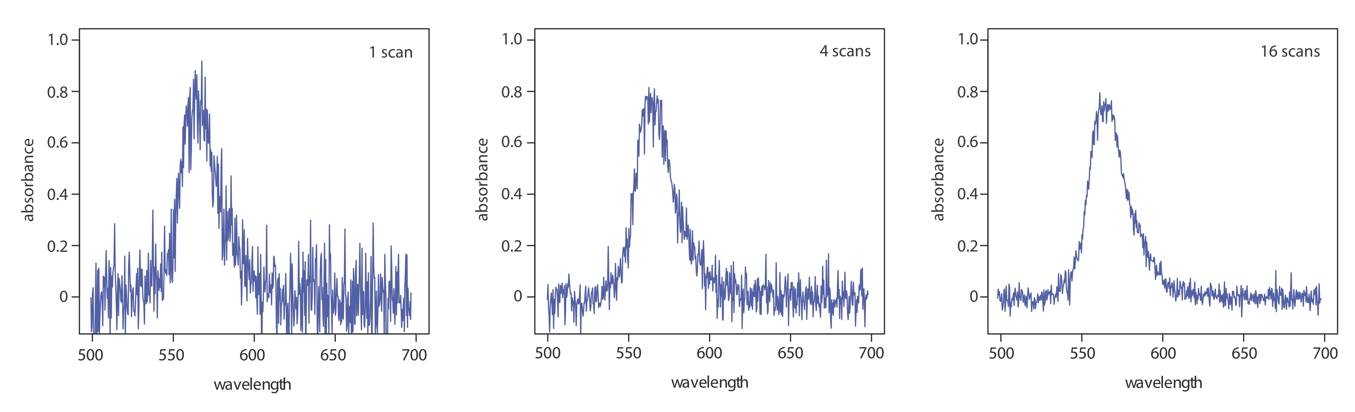
One advantage of a diode array spectrometer is the speed of data acquisition, which allows us to collect multiple spectra for a single sample. Individual spectra are added and averaged to obtain the final spectrum. This signal averaging improves a spectrum’s signal-to-noise ratio. If we add together n spectra, the sum of the signal at any point, x, increases as nS_x, where S_x is the signal. The noise at any point, N_x, is a random event, which increases as \(\sqrt{n} N_x\) when we add together n spectra. The signal-to-noise ratio after n scans, (S/N)_n is

\[\left(\frac{S}{N}\right)_{n}=\frac{n S_{x}}{\sqrt{n} N_{x}}=\sqrt{n} \frac{S_{x}}{N_{x}} \nonumber\]

where S_x/N_x is the signal-to-noise ratio for a single scan. The impact of signal averaging is shown in Figure 3.3.5 . The first spectrum shows the signal after one scan, which consists of a single, noisy peak. Signal averaging using 4 scans and 16 scans decreases the noise and improves the signal-to-noise ratio. One disadvantage of a photodiode array is that the effective bandwidth per diode is roughly an order of magnitude larger than that for a high quality monochromator.

Figure 3.3.5 . Effect of signal averaging on a spectrum’s signal-to-noise ratio. From top to bottom: spectrum for a single scan; average spectrum after four scans; and average spectrum after adding 16 scans.

For more details on signals and noise, see Introduction to Signals and Noise by Steven Petrovic, an on-line resource that is part of the Analytical Sciences Digital Library.

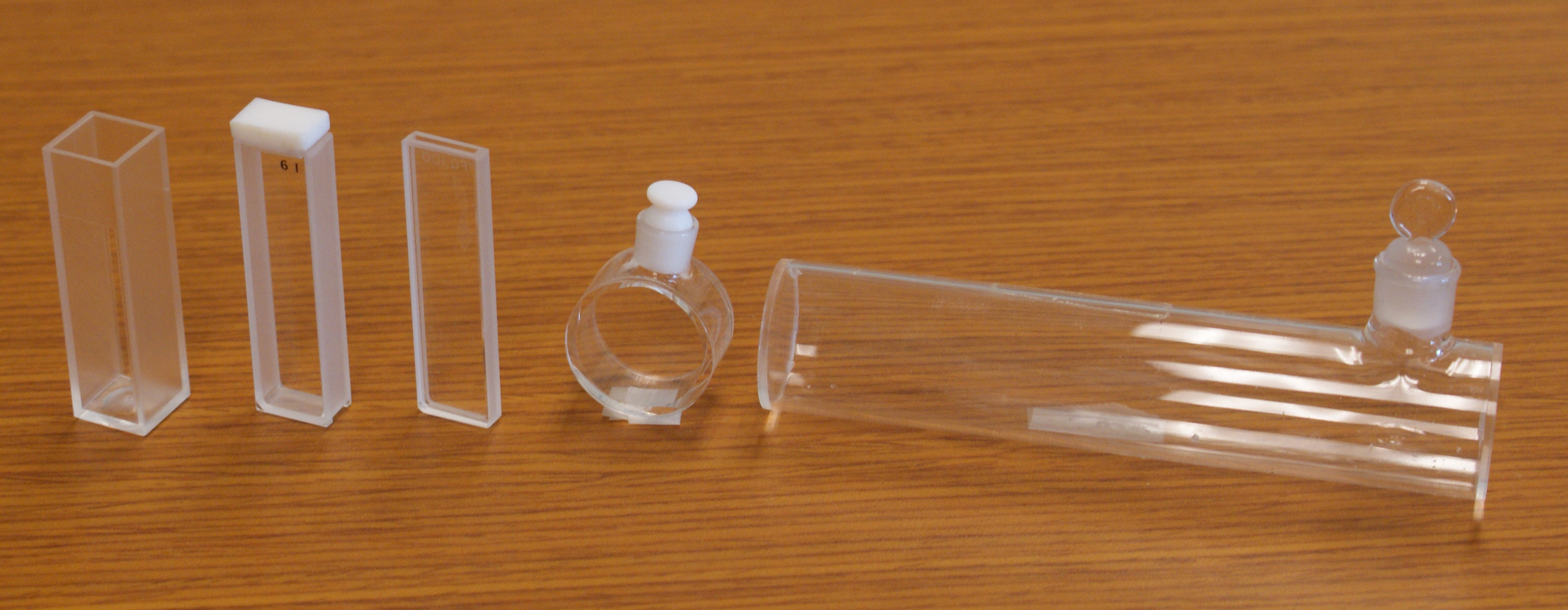
Sample Cells.

Samples that are in liquid or solution state are places in cells (called cuvettes) constructed with materials that are transparent to UV and/or Visible light. Common cuvette materials are quartz (fused silica), glass, and plastic (Figure 3.3.6 ). Glass and plastic are inexpensive, and they can be useful for analysis of samples that require the cell to be transparent only to visible light. However, glass is not transparent to light below about 380 nm. Some plastics are also not transparent to UV light. On the other hand, Quartz (or fused silica) is more expensive, but it is transparent to both UV and visible light. A quartz or fused-silica cell is required when working at a wavelength <300 nm where other materials show a significant absorption.

By far, the most common pathlength is 1 cm (10 mm), as is the case for the "standard" size cuvette pictured at the far left of Figure 3.3.6 . Cells with shorter (as little as 0.1 cm) and longer pathlengths (up to 10 cm) are also available. Longer pathlength cells are useful when analyzing a very dilute solution or for gas samples. The highest quality cells allow the radiation to strike a flat surface at a 90^o angle, minimizing the loss of radiation to reflection. A test tube often is used as a sample cell with simple, single-beam instruments, although differences in the cell’s pathlength and optical properties add an additional source of error to the analysis.

Figure 3.3.6 . Examples of sample cells for UV/Vis spectroscopy. From left to right (with path lengths in parentheses): rectangular plastic cuvette (10.0 mm), rectangular quartz cuvette (5.000 mm), rectangular quartz cuvette (1.000 mm), cylindrical quartz cuvette (10.00 mm), cylindrical glass cuvette with quartz windows (100.0 mm). Cells often are available as a matched pair, which is important when using a double-beam instrument.

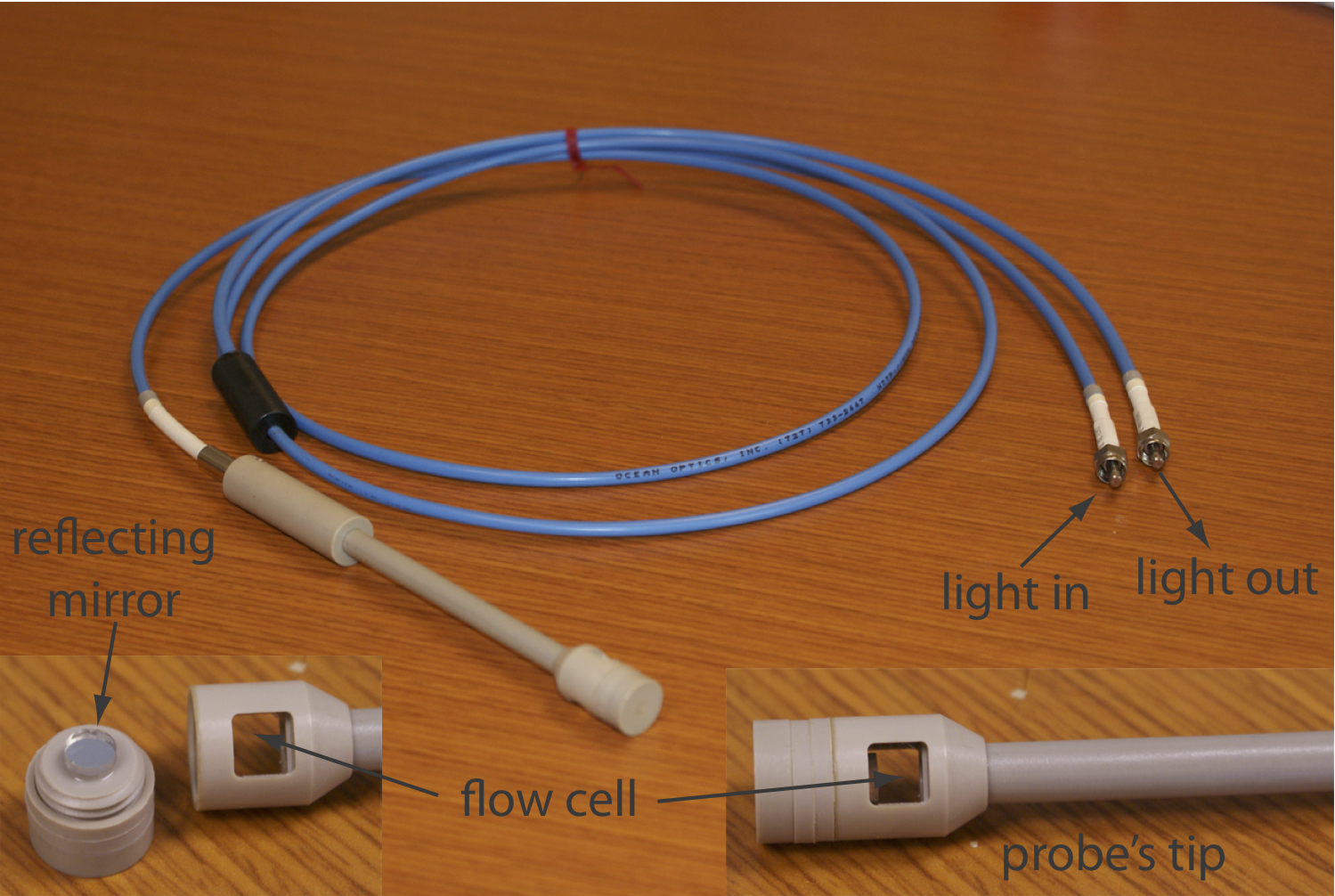
If we need to monitor an analyte’s concentration over time, it may not be possible to remove samples for analysis. This often is the case, for example, when monitoring an industrial production line or waste line, when monitoring a patient’s blood, or when monitoring an environmental system, such as stream. With a fiber-optic probe we can analyze samples in situ. An example of a remote sensing fiber-optic probe is shown in Figure 3.3.7 . The probe consists of two bundles of fiber-optic cable. One bundle transmits radiation from the source to the probe’s tip, which is designed to allow the sample to flow through the sample cell. Radiation from the source passes through the solution and is reflected back by a mirror. The second bundle of fiber-optic cable transmits the nonabsorbed radiation to the wavelength selector. Another design replaces the flow cell shown in Figure 3.3.7 with a membrane that contains a reagent that reacts with the analyte. When the analyte diffuses into the membrane it reacts with the reagent, producing a product that absorbs UV or visible radiation. The nonabsorbed radiation from the source is reflected or scattered back to the detector. Fiber optic probes that show chemical selectivity are called optrodes [(a) Seitz, W. R. Anal. Chem. 1984, 56, 16A–34A; (b) Angel, S. M. Spectroscopy 1987, 2(2), 38–48].

Figure 3.3.7 . Example of a fiber-optic probe. The inset photographs at the bottom of the figure provide close-up views of the probe’s flow cell and the reflecting mirror.

Evaluation of UV/Vis and IR Spectroscopy

Accuracy

Under normal conditions a relative error of 1–5% is easy to obtained with UV/Vis absorption. Accuracy usually is limited by the quality of the blank. Examples of the type of problems that are encountered include the pres- ence of particulates in the sample that scatter radiation, and the presence of interferents that react with analytical reagents. In the latter case the interferent may react to form an absorbing species, which leads to a positive determinate error. Interferents also may prevent the analyte from reacting, which leads to a negative determinate error. With care, it is possible to improve the accuracy of an analysis by as much as an order of magnitude.

Precision

In absorption spectroscopy, precision is limited by indeterminate errors—primarily instrumental noise—which are introduced when we measure absorbance. Precision generally is worse for low absorbances where P₀ ≈ P_T, and for high absorbances where P_T approaches 0. We might expect, therefore, that precision will vary with transmittance.

We can derive an expression between precision and transmittance by applying the propagation of uncertainty as described in Chapter 4. To do so we rewrite Beer’s law as

\[C=-\frac{1}{\varepsilon b} \log T \label{10.12}\]

Table 4.3.1 in Chapter 4 helps us complete the propagation of uncertainty for Equation \ref{10.12}; thus, the absolute uncertainty in the concentration, s_C, is

\[s_{c}=-\frac{0.4343}{\varepsilon b} \times \frac{s_{T}}{T} \label{10.13}\]

where s_T is the absolute uncertainty in the transmittance. Dividing Equation \ref{10.13} by Equation \ref{10.12} gives the relative uncertainty in concentration, s_C/C, as

\[\frac{s_c}{C}=\frac{0.4343 s_{T}}{T \log T} \nonumber\]

If we know the transmittance’s absolute uncertainty, then we can determine the relative uncertainty in concentration for any measured transmittance.

Determining the relative uncertainty in concentration is complicated because s_T is a function of the transmittance. As shown in Table 3.3.3 , three categories of indeterminate instrumental error are observed [Rothman, L. D.; Crouch, S. R.; Ingle, J. D. Jr. Anal. Chem. 1975, 47, 1226–1233]. A constant s_T is observed for the uncertainty associated with reading %T on a meter’s analog or digital scale. Typical values are ±0.2–0.3% (a k₁ of ±0.002–0.003) for an analog scale and ±0.001% a (k₁ of ±0.00001) for a digital scale.

Table 3.3.3 . Effect of Indeterminate Errors on Relative Uncertainty in Concentration

category	sources of indeterminate error	relative uncertainty in concentration
\(s_T = k_1\)	%T readout resolution noise in thermal detectors	\(\frac{s_{C}}{C}=\frac{0.4343 k_{1}}{T \log T}\)
\(s_T = k_2 \sqrt{T^2 + T}\)	noise in photon detectors	\(\frac{s_{C}}{C}=\frac{0.4343 k_{2}}{\log T} \sqrt{1+\frac{1}{T}}\)
\(s_T = k_3 T\)	positioning of sample cell fluctuations in source intensity	\(\frac{s_{C}}{C}=\frac{0.4343 k_{3}}{\log T}\)

A constant s_T also is observed for the thermal transducers used in infrared spectrophotometers. The effect of a constant s_T on the relative uncertainty in concentration is shown by curve A in Figure 3.3.16 . Note that the relative uncertainty is very large for both high absorbances and low absorbances, reaching a minimum when the absorbance is 0.4343. This source of indeterminate error is important for infrared spectrophotometers and for inexpensive UV/Vis spectrophotometers. To obtain a relative uncertainty in concentration of ±1–2%, the absorbance is kept within the range 0.1–1.

Figure 3.3.16 . Percent relative uncertainty in concentration as a function of absorbance for the categories of indeterminate errors in Table \(\PageIndex{10.3}\). A: k₁ = ±0.0030; B: k₂ = ±0.0030; and C: k₃= ±0.0130. The dashed lines correspond to the minimum uncertainty for curve A (absorbance of 0.4343) and for curve B (absorbance of 0.963).

Values of s_T are a complex function of transmittance when indeterminate errors are dominated by the noise associated with photon detectors. Curve B in Figure 3.3.16 shows that the relative uncertainty in concentration is very large for low absorbances, but is smaller at higher absorbances. Although the relative uncertainty reaches a minimum when the absorbance is 0.963, there is little change in the relative uncertainty for absorbances between 0.5 and 2. This source of indeterminate error generally limits the precision of high quality UV/Vis spectrophotometers for mid-to-high absorbances.

Finally, the value of s_T is directly proportional to transmittance for indeterminate errors that result from fluctuations in the source’s intensity and from uncertainty in positioning the sample within the spectrometer. The latter is particularly important because the optical properties of a sample cell are not uniform. As a result, repositioning the sample cell may lead to a change in the intensity of transmitted radiation. As shown by curve C in Figure 3.3.16 , the effect is important only at low absorbances. This source of indeterminate errors usually is the limiting factor for high quality UV/Vis spectrophotometers when the absorbance is relatively small.

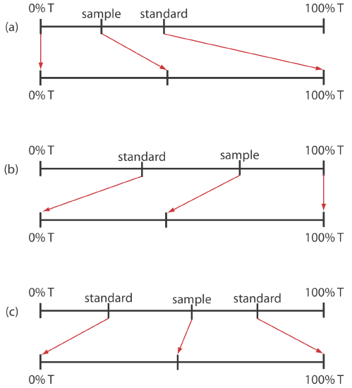
When the relative uncertainty in concentration is limited by the %T readout resolution, it is possible to improve the precision of the analysis by redefining 100% T and 0% T. Normally 100% T is established using a blank and 0% T is established while preventing the source’s radiation from reaching the detector. If the absorbance is too high, precision is improved by resetting 100% T using a standard solution of analyte whose concentration is less than that of the sample (Figure 3.3.17 a). For a sample whose absorbance is too low, precision is improved by redefining 0% T using a standard solution of the analyte whose concentration is greater than that of the analyte (Figure 3.3.17 b). In this case a calibration curve is required because a linear relationship between absorbance and concentration no longer exists. Precision is further increased by combining these two methods (Figure 3.3.17 c). Again, a calibration curve is necessary since the relation- ship between absorbance and concentration is no longer linear.

Figure 3.3.17 . Methods for improving the precision of absorption methods: (a) high-absorbance method; (b) low-absorbance method; (c) maximum precision method.

Sensitivity

The sensitivity of a molecular absorption method, which is the slope of a Beer’s law calibration curve, is the product of the analyte’s absorptivity and the pathlength of the sample cell (\(\varepsilon b\)). You can improve a method’s sensitivity by selecting a wavelength where absorbance is at a maximum or by increasing pathlength.

See Figure 10.2.10 for an example of how the choice of wavelength affects a calibration curve’s sensitivity.

Selectivity

Selectivity rarely is a problem in molecular absorption spectrophotometry. In many cases it is possible to find a wavelength where only the analyte absorbs. When two or more species do contribute to the measured absorbance, a multicomponent analysis is still possible, as shown in Example 3.3.2 and Example 3.3.3 .

Time, Cost, and Equipment

The analysis of a sample by molecular absorption spectroscopy is relatively rapid, although additional time is required if we need to convert a nonabsorbing analyte into an absorbing form. The cost of UV/Vis instrumentation ranges from several hundred dollars for a simple filter photometer, to more than $50,000 for a computer-controlled, high-resolution double-beam instrument equipped with variable slit widths, and operating over an extended range of wavelengths. Fourier transform infrared spectrometers can be obtained for as little as $15,000–$20,000, although more expensive models are available.