2.4: Methods of Calibration

Single Point Calibration vs Multiple-point Calibration

The simplest calibration is a single-point calibration using a standard. For example, using a standard solution of known concentration of component \(X\), we could measure its signal (eg absorption), and then calculate the response (eg the \(\varepsilon_{X}\) at the wavelength of maximum absorbance).

Limitations to Single-point calibration

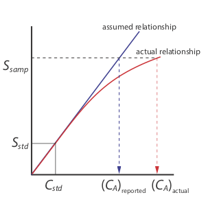
A single-point standardization is the least desirable approach for standardizing a method. There are two reasons for this. First, any error in our determination of the response, (eg \(\varepsilon_{X}\)), carries over into our calculation of concentratino (\(C_{X}\)). Second, our experimental value for each response (eg \(\varepsilon\)) is based on a single concentration of analyte. To extend this value of \(\varepsilon\) to other concentrations of analyte requires that we assume a linear relationship between the signal and the analyte’s concentration, an assumption that often is not true [Cardone, M. J.; Palmero, P. J.; Sybrandt, L. B. Anal. Chem. 1980, 52, 1187–1191]. Figure 2.4.1 shows how assuming a constant value of response leads to a determinate error in concentration if \the response becomes smaller at higher concentrations of analyte. Despite these limitations, single-point standardizations find routine use when the expected range for the analyte’s concentrations is small.

Figure 2.4.1 : Example showing how a single-point standardization leads to a determinate error in an analyte’s reported concentration if we incorrectly assume that the response (slope) is constant. The assumed relationship between the sample signal (\(S_{samp}\)) and concentration of the analyte \((C_A\)) is based on a single standard and is a straight-line; the actual relationship between \(S_{samp}\) and \(C_A\) becomes curved for larger concentrations of analyte.

Multi-point Calibration

The better way to standardize a method is to prepare a series of standards, each of which contains a different concentration of analyte. Standards are chosen such that they bracket the expected range for the analyte’s concentration. A multiple-point standardization should include at least three standards, although more are preferable. A plot of the signal from the standards (\(S_{std}\) versus the concentrations of the standards (\(C_{std}\)) is called a calibration curve. The exact standardization, or calibration relationship, is determined by an appropriate curve-fitting algorithm.

There are two advantages to a multiple-point standardization. First, although a determinate error in one standard introduces a determinate error, its effect is minimized by the remaining standards. Second, because we measure the signal for several concentrations of analyte, we no longer must assume that the response (\(\varepsilon\) in this case) is independent of the analyte’s concentration. Instead, we can construct a calibration curve similar to the “actual relationship” indicated in Figure 2.4.1 .

External Calibration

The most common method of standardization uses one or more external standards, each of which contains a known concentration of analyte. We call these standards “external” because they are prepared and analyzed separate from the samples.

Figure 2.4.2 shows a typical multiple-point external standardization. The volumetric flask on the left contains a reagent blank and the remaining volumetric flasks contain increasing concentrations of Cu²⁺. Shown below the volumetric flasks is the resulting calibration curve. Because this is the most common method of standardization, the resulting relationship is called a normal calibration curve.

Figure 2.4.2 : The photo at the top of the figure shows a reagent blank (far left) and a set of five external standards for Cu²⁺ with concentrations that increase from left-to-right. Shown below the external standards is the resulting normal calibration curve. The absorbance signal of each standard, \(S_{std}\) is shown by the filled circles.

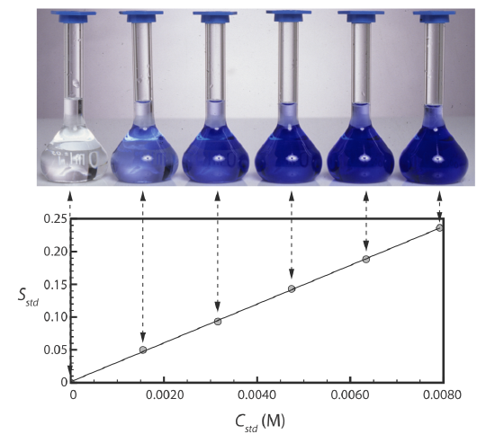
When a calibration curve is a straight-line, as it is in Figure 2.4.2 , the slope of the line gives the value of \(b\varepsilon\) (where \(b\) is path length) This is the most desirable situation because the method’s sensitivity remains constant throughout the analyte’s concentration range. When the calibration curve is not a straight-line, the method’s sensitivity is a function of the analyte’s concentration. In Figure 2.4.1 , for example, the value of \(b\varepsilon\) is greatest when the analyte’s concentration is small and it decreases continuously for higher concentrations of analyte. The value of \(b\varepsilon\) at any point along the calibration curve in Figure 2.4.1 is the slope at that point. In either case, a calibration curve allows us to relate \(S_{samp}\) to the analyte’s concentration.

Limitations to External Calibration

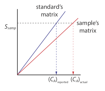
There is a serious limitation, however, to an external standardization. When we determine and analyte's response (\\varepsilon\) in this case) using external calibration, the analyte is present in the external standard’s matrix; that is usually a much simpler matrix than that of "real" samples. When we use an external standardization we assume the matrix does not affect the value of the response (\(\varepsilon\)). However, if the matrix does affect the response, we introduce a proportional determinate error into our analysis. This is not the case in Figure 2.4.3 , for instance, where we show calibration curves for an analyte in the sample’s matrix and in the standard’s matrix. In this case, using the calibration curve for the external standards leads to a negative determinate error in analyte’s reported concentration. If we expect that matrix effects are important, then we try to match the standard’s matrix to that of the sample, a process known as matrix matching. If we are unsure of the sample’s matrix, then we must show that matrix effects are negligible or use an alternative method of standardization. Both approaches are discussed in the following section.

Figure 2.4.3 : Calibration curves for an analyte in the standard’s matrix and in the sample’s matrix. If the matrix affects the response (slope) as is the case here, then we introduce a proportional determinate error into our analysis if we use a normal calibration curve.

Validating an external calibration

 

Calibration by Standard Additions

We can avoid the complication of matching the matrix of the standards to the matrix of the sample if we carry out the standardization in the sample. This is known as the method of standard additions.

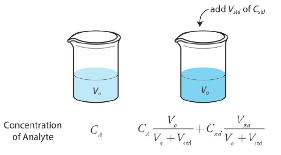
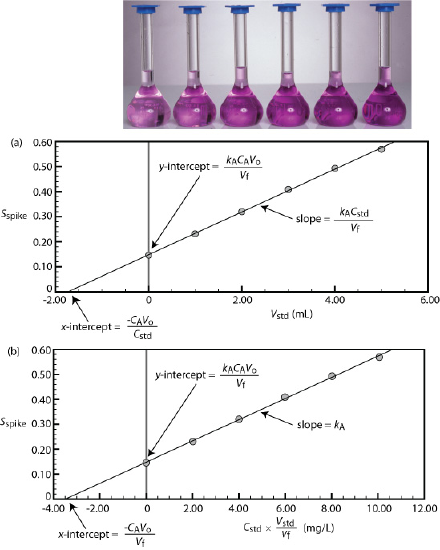
There are several methods of standard addition, and some are described in detail in 5.3: Determining the Sensitivity by David Harvey. We will focus on standard addition by adding standard analyte solution directly to the sample, measuring the signal both before and after the spike (Figure 2.4.5 ). In this case the final volume after the standard addition is V_o + V_std and the relationship between the absorbance and concentration of a analyte "X" becomes (the standard is a standard solution of the analyte X):

\[A_{sample} = \varepsilon b C_X \nonumber\]

\[A_{spiked} = \varepsilon b \left( C_X \frac {V_o} {V_o + V_{std}} + C_{std} \frac {V_{std}} {V_o + V_{std}} \right) \label{5.10}\]

\[\frac {A_{sample}} {C_X} = \frac {A_{spiked}} {C_X \frac {V_o} {V_o + V_{std}} + C_{std} \frac {V_{std}} {V_o + V_{std}}} \label{5.11}\]

Figure 2.4.5 : Illustration showing an alternative form of the method of standard additions. In this case we add the spike of external standard directly to the sample without any further adjust in the volume.

Multiple Standard Additions

We can adapt a single-point standard addition into a multiple-point standard addition by preparing a series of samples that contain increasing amounts of the external standard. Figure 2.4.6 shows two ways to plot a standard addition calibration curve based on equation \ref{5.10}. In Figure 2.4.6 , plot (a) we plot A_spike (or more generally S_spike) against the volume of the spikes, V_std. In plot (b) we plot \(C_{std}\times \frac{V_{std}}{V_f}\) on the x axis instead (where \(V_f=V_{0}+V_{std}\) is total volume after the spike). If k_A is constant, then the calibration curve is a straight line in both cases. It is easy to show that the slope is related to the response of the analyte in the given matrix (\(k_A\) and that x-intercept is related to the concentration of the analyte \(C_A\); the x-intercept is equivalent to \(\frac{–C_A V_o}{C_{std}} \) in the case of plot (a) or \(\frac{–C_A V_o}{V_f} \) in the case of plot (b) (see Figure 2.4.6 ).

Figure 2.4.6 : Shown at the top of the figure is a set of six standard additions for the determination of Mn²⁺. The flask on the left is a 25.00 mL sample diluted to 50.00 mL with water. The remaining flasks contain 25.00 mL of sample and, from left-to-right, 1.00, 2.00, 3.00, 4.00, and 5.00 mL spikes of an external standard that is 100.6 mg/L Mn²⁺. Shown below are two ways to plot the standard additions calibration curve. The absorbance for each standard addition, S_spike, is shown by the filled circles.

For Mixtures with overlapping signals: The two-analyte Generalized Standard Addition Method (GSAM)

Suppose we need to determine the concentration of two analytes, X and Y, that are mixed in a sample. If each analyte has a wavelength where the other analyte does not absorb, then we can proceed using Beer's Law to determine the concentration. Unfortunately, UV/Vis absorption bands are so broad that it is sometimes impossible to find suitable wavelengths. Because Beer’s law is additive the mixture’s absorbance, A_mix, at a given wavelength will be a sum of the absorbance of each analyte:

\[\left(A_{m i x}\right)_{\lambda_{1}}=\left(\varepsilon_{X}\right)_{\lambda_{1}} b C_{X}+\left(\varepsilon_{Y}\right)_{\lambda_{1}} b C_{Y} \label{10.1}\]

where \(\lambda_1\) is the wavelength at which we measure the absorbance. Because Equation \ref{10.1} includes terms for the concentration of both X and Y, the absorbance at one wavelength does not provide enough information to determine either C_X or C_Y. If we measure the absorbance at a second wavelength, \(\lambda_2\)

\[\left(A_{m i x}\right)_{\lambda_{2}}=\left(\varepsilon_{x}\right)_{\lambda_{2}} b C_{X}+\left(\varepsilon_{Y}\right)_{\lambda_{2}} b C_{Y} \label{10.2}\]

then we can determine C_X and C_Y by solving simultaneously Equation \ref{10.1} and Equation \ref{10.2}. Of course, we also must determine the value for \(\varepsilon_X\) and \(\varepsilon_Y\) at each wavelength. For a mixture of n components, we must measure the absorbance at n different wavelengths.

Example 2.4.1

The concentrations of Fe³⁺ and Cu²⁺ in a mixture are determined following their reaction with hexacyanoruthenate (II), \(\text{Ru(CN)}_6^{4-}\), which forms a purple-blue complex with Fe³⁺ (\(\lambda_\text{max}\) = 550 nm) and a pale-green complex with Cu²⁺ (\(\lambda_\text{max}\) = 396 nm) [DiTusa, M. R.; Schlit, A. A. J. Chem. Educ. 1985, 62, 541–542]. The molar absorptivities (M^–1 cm^–1) for the solutions of the individual metal complexes at the two wavelengths are summarized in the following table.

analyte	\(\varepsilon_{550}\)	\(\varepsilon_{396}\)
Fe^3^+standard	9970	84
Cu^2^+ standard	34	856

When a sample that contains Fe³⁺ and Cu²⁺ is analyzed in a cell with a pathlength of 1.00 cm, the absorbance at 550 nm is 0.183 and the absorbance at 396 nm is 0.109. What are the molar concentrations of Fe³⁺ and Cu²⁺ in the sample?

Solution

Substituting known values into Equation \ref{10.1} and Equation \ref{10.2} gives

\[\begin{aligned} A_{550} &=0.183=9970 C_{\mathrm{Fe}}+34 C_{\mathrm{Cu}} \\ A_{396} &=0.109=84 C_{\mathrm{Fe}}+856 C_{\mathrm{Cu}} \end{aligned} \nonumber\]

To determine C_Fe and C_Cu we solve the first equation for C_Cu

\[C_{\mathrm{Cu}}=\frac{0.183-9970 C_{\mathrm{Fe}}}{34} \nonumber\]

and substitute the result into the second equation.

\[\begin{aligned} 0.109 &=84 C_{\mathrm{Fe}}+856 \times \frac{0.183-9970 C_{\mathrm{Fe}}}{34} \\ &=4.607-\left(2.51 \times 10^{5}\right) C_{\mathrm{Fe}} \end{aligned} \nonumber\]

Solving for C_Fe gives the concentration of Fe³⁺ as \(1.8 \times 10^{-5}\) M. Substituting this concentration back into the equation for the mixture’s absorbance at 396 nm gives the concentration of Cu²⁺ as \(1.3 \times 10^{-4}\) M.

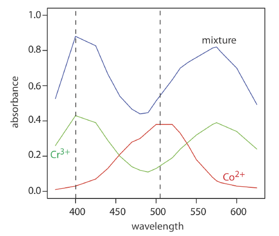
Let's consider the example of a mixed Co and Cr solution. To obtain results with good accuracy and precision the two wavelengths should be selected so that \(\varepsilon_X > \varepsilon_Y\) at one wavelength and \(\varepsilon_X < \varepsilon_Y\) at the other wavelength. It is easy to appreciate why this is true. Because the absorbance at each wavelength is dominated by one analyte, any uncertainty in the concentration of the other analyte has less of an impact. Figure 2.4.1 shows the spectra of a Cr standard and a Co standard, as well as a spectrum of the mixture. From the spectra of the standards, we can see that 400 nm is a reasonable choice for one of the wavelengths because it is a point of maximum absorption for \(\ce{Cr^3+}\), and \(\varepsilon_{Cr}\) > \(\varepsilon_{Co}\). A reasonable choice for a second wavelength is 505 nm; it is a point of maximum absorbance for \(\ce{Co^2+}\) where \(\varepsilon_{Co}\) > \(\varepsilon_{Cr}\). These two wavelengths are used in Practice Exercise 2.4.1 (below). When the choice of wavelengths is not obvious, one method for locating the optimum wavelengths is to plot \(\varepsilon_X / \varepsilon_y\) as function of wavelength, and determine the wavelengths where \(\varepsilon_X / \varepsilon_y\) reaches maximum and minimum values [Mehra, M. C.; Rioux, J. J. Chem. Educ. 1982, 59, 688–689].

Figure 2.4.1 . Visible absorption spectra for 0.0250 M Cr³⁺, 0.0750 M Co²⁺, and for a mixture of Cr³⁺ and Co²⁺. The two wavelengths used to analyze the mixture of Cr³⁺ and Co²⁺ are shown by the dashed lines. The data for the two standards are from Brewer, S. Solving Problems in Analytical Chemistry, John Wiley & Sons: New York, 1980.

Exercise 2.4.1

The absorbance spectra for Cr³⁺ and Co²⁺ overlap significantly. To determine the concentration of these analytes in a mixture, its absorbance is measured at 400 nm and at 505 nm, yielding values of 0.336 and 0.187, respectively. The individual molar absorptivities (M^–1 cm^–1) for Cr3⁺ are 15.2 at 400 nm and 0.533 at 505 nm; the values for Co²⁺ are 5.60 at 400 nm and 5.07 at 505 nm.

Answer

Substituting into Equation \ref{10.1} and Equation \ref{10.2} gives

\[A_{400} = 0.336 = 15.2C_\text{Cr} + 5.60C_\text{Co} \nonumber\]

\[A_{400} = 0187 = 0.533C_\text{Cr} + 5.07C_\text{Co} \nonumber\]

To determine C_Cr and C_Co we solve the first equation for C_Co

\[C_{\mathrm{Co}}=\frac{0.336-15.2 \mathrm{C}_{\mathrm{Co}}}{5.60} \nonumber\]

and substitute the result into the second equation.

\[0.187=0.533 C_{\mathrm{Cr}}+5.07 \times \frac{0.336-15.2 C_{\mathrm{Co}}}{5.60} \nonumber\]

\[0.187=0.3042-13.23 C_{\mathrm{Cr}} \nonumber\]

Solving for C_Cr gives the concentration of Cr³⁺ as \(8.86 \times 10^{-3}\) M. Substituting this concentration back into the equation for the mixture’s absorbance at 400 nm gives the concentration of Co²⁺ as \(3.60 \times 10^{-2}\) M.

 

We can extend the standard addition method to quantitate multiple components of a mixture using the Generalized Standard Addition Method (GSAM). This is the preferred method of calibration when quantitation of multiple components are necessary and matrix effects are suspected. This is the method you will use to quantitate two components of a mixture (eg Co and Cr) that have overlapping spectral features (see Figure 3.4.1) and when matrix effects are suspected. For a sample with components X and Y, the initial absorbance of the sample at \(\lambda_1\) is:

\[A_{\lambda_1}^0 = \varepsilon_{X_{\lambda_1}} b C_X^0 + \varepsilon_{Y_{\lambda_1}} b C_Y^0 \label{1} \]

Where \(\varepsilon_{X_{\lambda_1}}\) is the response factor (aka sensitivity, molar extinction coefficient, or the molar absorptivity) for component X at \(\lambda_1\), and \(\varepsilon_{Y_{\lambda_1}}\) is the response factor for component Y at \(\lambda_1\).

In this method, the volume of total sample will change as standard solution of X or Y is added to the sample to create the standard addition calibration for X and Y. When volume changes, concentrations are not additive. But we can correct for this inconvenient truth by multiplying by total volume, \(V_t\). When C is multiplied by V, the result is total moles (\(n\)) of each analyte; this value is additive. Multiplying by V gives the equation below.

\[V^0A_{\lambda_1}^0 = \varepsilon_{X_{\lambda_1}} b n_X^0 + \varepsilon_{Y_{\lambda_1}} b n_Y^0 \label{2} \]

As standards are added to the sample to create the calibration, the moles of analyte will change by \(\Delta n_x\) and \(\Delta n_y\), and the new volume-corrected absorption for any point on the calibration would be:

\[V^iA_{\lambda_1}^i = \varepsilon_{X_{\lambda_1}} b(\Delta n_x+ n_X^0) + \varepsilon_{Y_{\lambda_1}} b (\Delta n_Y + n_Y^0) \label{3}\]

where \(\Delta n_X\) is the moles of X added and \(n_X^0\) is the initial amount of analyte in the sample. The same follows for analyte Y.

The initial volume-corrected absorption, \(V^0A^0\) (Equation \ref{2}) can be factored from Equation \ref{3} to give the change in absorbance upon standard addition:

\[\Delta (VA_{\lambda_1}) = V^iA_{\lambda_1}^i - V^0A_{\lambda_1}^0 = \varepsilon_{X_{\lambda_1}} b(\Delta n_X) + \varepsilon_{Y_{\lambda_1}} b (\Delta n_Y) \label{4}\]

For a mixture of two analytes, absorbance would be measured at two wavelengths as described above. The same model described here for \(\lambda_1\), also applies for \(\lambda_2\):

\[\Delta (VA_{\lambda_2}) = V^iA_{\lambda_2}^i - V^0A_{\lambda_2}^0 = \varepsilon_{X_{\lambda_2}} b(\Delta n_X) + \varepsilon_{Y_{\lambda_2}} b (\Delta n_Y) \label{5}\]

Using a known volume of the sample, we can add known amounts of one analyte to the solution to create a calibration line with at least 3 points. For example, suppose we have a sample containing  two analytes, X, and Y in a complex matrix where matrix effects are unknown; and suppose we want to determine the concentrations of [X] and [Y] in the sample. This is a problem that can be solved by GSAM. First, we would obtain standard solutions of X and Y, collect their absorption spectra, and select appropriate wavelengths for analysis. Then, we would collect a spectrum of the analyte solution containing unknown amounts of X and Y.

To create a standard curve for X, we could add a standard solution of X into a known quantity of the sample while monitoring the solution mixture at the two wavelengths. Under these conditions, \(\Delta n_Y\) is zero, and so equation \ref{4} is simplified to a \(\Delta (VA_{\lambda_1}) = \varepsilon_{X_{\lambda_1}} b(\Delta n_X)\) ; this is the form of a linear equation with the slope that is \(\varepsilon_{X_{\lambda_1}} b\). By plotting \(\Delta (VA_{\lambda_1})\) at one wavelength vs \(\Delta n_X\) we can determine the molar response factor of X at that wavelength (\(\varepsilon_{\lambda_1}\)). And, by plotting \(\Delta (VA_{\lambda_2})\) at the second wavelength vs \(\Delta n_X\) we can determine the molar response factor of X at the second wavelength (\(\varepsilon_{\lambda_2}\)). 

Then, using the same sample as above, we can add two aliquots of Y and follow a similar strategy plotting \(\Delta n_Y\) against \(\Delta (VA_{\lambda_1})\) and \(\Delta (VA_{\lambda_2})\) to find the response factors of Y at the two wavelengths.

Once the response factors of both analytes X and Y are determined at the two different wavelengths, the concentrations of each analyte in the original sample can be determined by simultaneously solving equation \ref{1} and the analogous equation at \(\lambda_2\):

\[A_{\lambda_1}^0 = \varepsilon_{X_{\lambda_1}} b C_X^0 + \varepsilon_{Y_{ \lambda_1}} b C_Y^0 \qquad  \text{and} \qquad A_{\lambda_2}^0 = \varepsilon_{X_{ \lambda_2}} b C_X^0 + \varepsilon_Y b C_{Y_{ \lambda_2}}^0 \label{6} \]