2.5: Uncertainty in values determined from a Calibration Curve

You learned how to propogate error in the prerequisite laboratory courses, CHEM301L or CHEM310L; thus, if you are here, we expect you know the sources of experimental error and how to propagate of errors in measurements (review as necessary). However, when we determine an analyte concentration from a calibration curve (a linear regression), a simple propagation of error is not sufficient. You can read more about this in 5.4: Linear Regression and Calibration Curves by David Harvey. A brief summary is below.

Obtaining the Analyte's Concentration From a Regression Equation and determining error

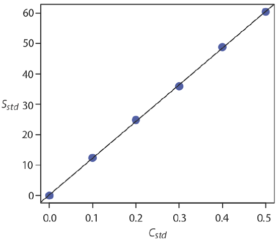
When a calibration curve is a straight-line, we represent it using the following mathematical equation

\[y = b + m x \label{5.1}\]

where y is the analyte’s signal, S_std, and x is the analyte’s concentration, C_std. The constants \(b\) and \(m\) are, respectively, the calibration curve’s expected y-intercept and its expected slope. An example of such a calibration curve is shown below in the figure.

Figure 2.5.1 : Calibration curve for the data in Table 2.5.1 and Example 2.5.1 .

Once we have our regression equation, it is easy to determine the concentration of analyte in a sample. When we use a normal calibration curve, for example, we measure the signal for our sample, S_samp, and calculate the analyte’s concentration, C_A, using the regression equation.

\[C_A = \frac {S_{samp} - b} {m} \label{5.11}\]

What is less obvious is how to report a confidence interval for C_A that expresses the uncertainty in our analysis. To calculate a confidence interval we need to know the standard deviation in the analyte’s concentration, \(s_{C_A}\), which is given by the following equation

\[s_{C_A} = \frac {s_r} {|m|} \sqrt{\frac {1} {k} + \frac {1} {n} + \frac {\left( S_{samp} - \overline{S}_{std} \right)^2} {m^2 \sum_{i = 1}^{n} \left( C_{std_i} - \overline{C}_{std} \right)^2}} \label{5.12}\]

where k is the number of replicate measurements we use to establish the sample’s average signal, S_samp, n is the number of calibration standards (the number of points in the calibration curve), S_std is the average signal for the calibration standards, and \(C_{std_1}\) and \(\overline{C}_{std}\) are the individual and the mean concentrations for the calibration standards. Knowing the value of \(s_{C_A}\), the confidence interval for the analyte’s concentration is

\[\mu_{C_A} = C_A \pm t s_{C_A} \nonumber\]

where \(\mu_{C_A}\) is the expected value of C_A in the absence of determinate errors, and with the value of t is based on the desired level of confidence and n – 2 degrees of freedom.

Equation \ref{5.12} is written in terms of a calibration experiment. A more general form of the equation, written in terms of x and y, is given below.

\[s_{x} = \frac {s_y} {|m|} \sqrt{\frac {1} {k} + \frac {1} {n} + \frac {\left( y - \overline{y} \right)^2} {m^2 \sum_{i = 1}^{n} \left( x_i - \overline{x} \right)^2}} \]

The same equation with all the variables labeled is shown in Figure \(\PageIndex{3}\).

A close examination of Equation \ref{5.12} should convince you that the uncertainty in C_A is smallest when the sample’s average signal, \(\overline{S}_{samp}\), is equal to the average signal for the standards, \(\overline{S}_{std}\). When practical, you should plan your calibration curve so that S_samp falls in the middle of the calibration curve. For more information about these regression equations see (a) Miller, J. N. Analyst 1991, 116, 3–14; (b) Sharaf, M. A.; Illman, D. L.; Kowalski, B. R. Chemometrics, Wiley-Interscience: New York, 1986, pp. 126-127; (c) Analytical Methods Committee “Uncertainties in concentrations estimated from calibration experiments,” AMC Technical Brief, March 2006.

Example 2.5.3

Three replicate analyses for a sample that contains an unknown concentration of analyte, yield values for S_samp of 29.32, 29.16 and 29.51 (arbitrary units). Using the results from Example 2.5.1 and Example 2.5.2 , determine the analyte’s concentration, C_A, and its 95% confidence interval.

Solution

The average signal, \(\overline{S}_{samp}\), is 29.33, which, using Equation \ref{5.11} and the slope and the y-intercept from Example 2.5.1 , gives the analyte’s concentration as

\[C_A = \frac {\overline{S}_{samp} - b} {m} = \frac {29.33 - 0.209} {120.706} = 0.241 \nonumber\]

To calculate the standard deviation for the analyte’s concentration we must determine the values for \(\overline{S}_{std}\) and for \(\sum_{i = 1}^{2} (C_{std_i} - \overline{C}_{std})^2\). The former is just the average signal for the calibration standards, which, using the data in Table 2.5.1 , is 30.385. Calculating \(\sum_{i = 1}^{2} (C_{std_i} - \overline{C}_{std})^2\) looks formidable, but we can simplify its calculation by recognizing that this sum-of-squares is the numerator in a standard deviation equation; thus,

\[\sum_{i = 1}^{n} (C_{std_i} - \overline{C}_{std})^2 = (s_{C_{std}})^2 \times (n - 1) \nonumber\]

where \(s_{C_{std}}\) is the standard deviation for the concentration of analyte in the calibration standards. Using the data in Table 2.5.1 we find that \(s_{C_{std}}\) is 0.1871 and

\[\sum_{i = 1}^{n} (C_{std_i} - \overline{C}_{std})^2 = (0.1872)^2 \times (6 - 1) = 0.175 \nonumber\]

Substituting known values into Equation \ref{5.12} gives

\[s_{C_A} = \frac {0.4035} {120.706} \sqrt{\frac {1} {3} + \frac {1} {6} + \frac {(29.33 - 30.385)^2} {(120.706)^2 \times 0.175}} = 0.0024 \nonumber\]

Finally, the 95% confidence interval for 4 degrees of freedom is

\[\mu_{C_A} = C_A \pm ts_{C_A} = 0.241 \pm (2.78 \times 0.0024) = 0.241 \pm 0.007 \nonumber\]

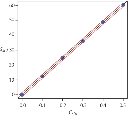
Figure 2.5.2 shows the calibration curve with curves showing the 95% confidence interval for C_A.

Figure 2.5.2 : Example of a normal calibration curve with a superimposed confidence interval for the analyte’s concentration. The points in blue are the original data from Table 2.5.1 . The black line is the normal calibration curve as determined in Example 2.5.1 . The red lines show the 95% confidence interval for C_A assuming a single determination of S_samp.

In a standard addition we determine the analyte’s concentration by extrapolating the calibration curve to the x-intercept. In this case the value of C_A is

\[C_A = x\text{-intercept} = \frac {-b} {m} \nonumber\]

and the standard deviation in C_A is

\[s_{C_A} = \frac {s_r} {m} \sqrt{\frac {1} {n} + \frac {(\overline{S}_{std})^2} {(m)^2 \sum_{i = 1}^{n}(C_{std_i} - \overline{C}_{std})^2}} \nonumber\]

where n is the number of standard additions (including the sample with no added standard), and \(\overline{S}_{std}\) is the average signal for the n standards. Because we determine the analyte’s concentration by extrapolation, rather than by interpolation, \(s_{C_A}\) for the method of standard additions generally is larger than for a normal calibration curve.

Exercise 2.5.1

Figure 2.5.2 shows a normal calibration curve for the quantitative analysis of Cu²⁺. The data for the calibration curve are shown here.

[Cu^2^+] (M)	Absorbance
0	0
\(1.55 \times 10^{-3}\)	0.050
\(3.16 \times 10^{-3}\)	0.093
\(4.74 \times 10^{-3}\)	0.143
\(6.34 \times 10^{-3}\)	0.188
\(7.92 \times 10^{-3}\)	0.236

Complete a linear regression analysis for this calibration data, reporting the calibration equation and the 95% confidence interval for the slope and the y-intercept. If three replicate samples give an S_samp of 0.114, what is the concentration of analyte in the sample and its 95% confidence interval?

Answer

We begin by setting up a table to help us organize the calculation

\(x_i\)	\(y_i\)	\(x_i y_i\)	\(x_i^2\)
0.000	0.000	0.000	0.000
\(1.55 \times 10^{-3}\)	0.050	\(7.750 \times 10^{-5}\)	\(2.403 \times 10^{-6}\)
\(3.16 \times 10^{-3}\)	0.093	\(2.939 \times 10^{-4}\)	\(9.986 \times 10^{-6}\)
\(4.74 \times 10^{-3}\)	0.143	\(6.778 \times 10^{-4}\)	\(2.247 \times 10^{-5}\)
\(6.34 \times 10^{-3}\)	0.188	\(1.192 \times 10^{-3}\)	\(4.020 \times 10^{-5}\)
\(7.92 \times 10^{-3}\)	0.236	\(1.869 \times 10^{-3}\)	\(6.273 \times 10^{-5}\)

Adding the values in each column gives

\[\sum_{i = 1}^{n} x_i = 2.371 \times 10^{-2} \quad \sum_{i = 1}^{n} y_i = 0.710 \quad \sum_{i = 1}^{n} x_i y_i = 4.110 \times 10^{-3} \quad \sum_{i = 1}^{n} x_i^2 = 1.378 \times 10^{-4} \nonumber\]

When we substitute these values into Equation \ref{5.4} and Equation \ref{5.5}, we find that the slope and the y-intercept are

\[m = \frac {6 \times (4.110 \times 10^{-3}) - (2.371 \times 10^{-2}) \times 0.710} {6 \times (1.378 \times 10^{-4}) - (2.371 \times 10^{-2})^2}) = 29.57 \nonumber\]

\[b = \frac {0.710 - 29.57 \times (2.371 \times 10^{-2}} {6} = 0.0015 \nonumber\]

and that the regression equation is

\[S_{std} = 29.57 \times C_{std} + 0.0015 \nonumber\]

To calculate the 95% confidence intervals, we first need to determine the standard deviation about the regression. The following table helps us organize the calculation.

\(x_i\)	\(y_i\)	\(\hat{y}_i\)	\((y_i - \hat{y}_i)^2\)
0.000	0.000	0.0015	\(2.250 \times 10^{-6}\)
\(1.55 \times 10^{-3}\)	0.050	0.0473	\(7.110 \times 10^{-6}\)
\(3.16 \times 10^{-3}\)	0.093	0.0949	\(3.768 \times 10^{-6}\)
\(4.74 \times 10^{-3}\)	0.143	0.1417	\(1.791 \times 10^{-6}\)
\(6.34 \times 10^{-3}\)	0.188	0.1890	\(9.483 \times 10^{-6}\)
\(7.92 \times 10^{-3}\)	0.236	0.2357	\(9.339 \times 10^{-6}\)

Adding together the data in the last column gives the numerator of Equation \ref{5.6} as \(1.596 \times 10^{-5}\). The standard deviation about the regression, therefore, is

\[s_r = \sqrt{\frac {1.596 \times 10^{-5}} {6 - 2}} = 1.997 \times 10^{-3} \nonumber\]

Next, we need to calculate the standard deviations for the slope and the y-intercept using Equation \ref{5.7} and Equation \ref{5.8}.

\[s_{m} = \sqrt{\frac {6 \times (1.997 \times 10^{-3})^2} {6 \times (1.378 \times 10^{-4}) - (2.371 \times 10^{-2})^2}} = 0.3007 \nonumber\]

\[s_{b} = \sqrt{\frac {(1.997 \times 10^{-3})^2 \times (1.378 \times 10^{-4})} {6 \times (1.378 \times 10^{-4}) - (2.371 \times 10^{-2})^2}} = 1.441 \times 10^{-3} \nonumber\]

and use them to calculate the 95% confidence intervals for the slope and the y-intercept

\[m = m \pm ts_{m} = 29.57 \pm (2.78 \times 0.3007) = 29.57 \text{ M}^{-1} \pm 0.84 \text{ M}^{-1} \nonumber\]

\[b = b \pm ts_{b} = 0.0015 \pm (2.78 \times 1.441 \times 10^{-3}) = 0.0015 \pm 0.0040 \nonumber\]

With an average S_samp of 0.114, the concentration of analyte, C_A, is

\[C_A = \frac {S_{samp} - b} {m} = \frac {0.114 - 0.0015} {29.57 \text{ M}^{-1}} = 3.80 \times 10^{-3} \text{ M} \nonumber\]

The standard deviation in C_A is

\[s_{C_A} = \frac {1.997 \times 10^{-3}} {29.57} \sqrt{\frac {1} {3} + \frac {1} {6} + \frac {(0.114 - 0.1183)^2} {(29.57)^2 \times (4.408 \times 10^{-5})}} = 4.778 \times 10^{-5} \nonumber\]

and the 95% confidence interval is

\[\mu = C_A \pm t s_{C_A} = 3.80 \times 10^{-3} \pm \{2.78 \times (4.778 \times 10^{-5})\} \nonumber\]

\[\mu = 3.80 \times 10^{-3} \text{ M} \pm 0.13 \times 10^{-3} \text{ M} \nonumber\]

Automate analysis using a calibration curve

You will create many calibration curves this semester, and you'll need to perform quality control checks to know whether your calibration curve is reasonable. The process of building a calibration curve, doing error analysis, and performing quality controls can become much more efficient when you build an automated tool to help you. In this example, we will use Excel. Below is an example of an excel spreadsheet template that you could build. Your TA's can help you through the creating of such a template. Alternatively, you could build your own script in MatLab or another data analysis software of your choice to perform the same functions. You can download an example to help get you started here: (Link for Duke Students).

Figure \(\PageIndex{3}\): This example was inspired by Harris's Qualitative Chemical Analysis textbook, Figure 4-15. After entering the correct formulas, you should find that the Derived x = 2.2325 and the \(s_x\) is 0.3735. (Kathryn Haas; CC-BY-SA)